Topic 6 · Dimensional Analysis

Solved Problems: Official Dimensional Analysis Sheets DA1 to DA14

Worked solutions to the fourteen dimensional-analysis sheets of the course, most of them past exam problems. Each statement is transcribed from the sheet and its figure redrawn; each solution follows the handwritten key of the sheet with every step written out: the list of governing parameters, the exponent matrix and the choice of the parameters with independent dimensions, every system of exponents solved, the limits Re ≫ 1 or Re ≪ 1, the conditions of physical similarity, the numbers and the tables converted from the model to the prototype, and the checks. Where the key has a slip, the correction is shown as an erratum. References to Notes.pdf are to Chapter 6 (Dimensional Analysis).

Problem DA1

Power of a Marine Freighter

Original statement · DA1.pdf
Π theoremFroude similarityRe ≫ 1

Official Problem Statement

We want to estimate the driving power $W$ necessary to move at a peak velocity $V = 10$ m/s a marine freighter of length $l = 100$ m and total mass at full load $m = 1000$ Tm. For that purpose, a small model of length $l_e = 1$ m, geometrically similar to the real ship, is to be tested on a hydraulic channel. To guide the design of the experiment, follow these steps:

1. Use the dimensional analysis to reduce the parametric dependence of the required power $W$.

2. Write the three equations that need to be satisfied to guarantee physical similarity between the experiment and the full-scale prototype. Verify that it is not possible to find the values of the mass $m_e$ and velocity $V_e$ of the experiment that satisfy simultaneously all three equations, so that complete physical similarity cannot be attained.

3. Assuming that the effect of viscosity on the fluid motion is negligible, determine the values of $m_e$ and $V_e$. Check that the corresponding values of the Reynolds number for both the real prototype and the experiment are indeed sufficiently large for the assumption of negligible viscosity to be a reasonable approximation.

4. If the experimental measurement of the power obtained with the experimental model is $W_e = 10$ W, obtain the value of the driving power $W$ needed to operate the real prototype at the required conditions.

Source: DA1.pdf (page 1, statement and handwritten key). Notes.pdf, Chapter 6: Π theorem, Eq. 6.25; physical similarity, Eqs. 6.57-6.59.

Worked solutionexpand / collapse

Hypotheses, Data and Dimensional Table

  • The ship moves at constant velocity on the free surface of water, which is the same liquid in the channel and in the sea: $\rho_e = \rho$, $\mu_e = \mu$, so $\nu_e = \nu = \mu/\rho \simeq 10^{-6}$ m$^2$/s.
  • The power goes into the waves made at the free surface (gravity $g$ matters, since the free surface is not flat; Notes.pdf, p. 66) and into the viscous drag ($\mu$ matters, a priori).
  • The mass $m$ fixes how deep the hull floats: by Archimedes, the submerged volume is $m/\rho$.
  • "Tm" is the metric ton: $m = 1000\ \text{t} = 10^6$ kg.
ParameterMeaningDimensionsValue (prototype)
$W$driving power (unknown)$ML^2T^{-3}$?
$V$ship velocity$LT^{-1}$10 m/s
$g$gravity$LT^{-2}$9.81 m/s$^2$
$m$mass at full load$M$$10^6$ kg
$l$ship length$L$100 m
$\rho$water density$ML^{-3}$1000 kg/m$^3$
$\mu$water viscosity$ML^{-1}T^{-1}$$10^{-3}$ kg/(m s)

Application of the Π Theorem

$$ W = W(V, g, m, l, \rho, \mu) $$

There are $n = 6$ governing parameters. Exponent matrix, rows $V$, $l$, $\rho$; columns $L$, $M$, $T$:

$$ \begin{pmatrix} 1 & 0 & -1 \\ 1 & 0 & 0 \\ -3 & 1 & 0 \end{pmatrix}, \qquad \det = 1\,(0\cdot 0 - 0\cdot 1) - 0 + (-1)\,(1\cdot 1 - 0\cdot(-3)) = -1 \neq 0 $$

so $(V, l, \rho)$ have independent dimensions and $k = 3$: there are $n - k = 3$ dimensionless parameters. $(V, l, \rho)$ is chosen because velocity, size and the inertia of the water clearly matter (Notes.pdf, p. 68).

Power. $[W] = [\rho]^a[V]^b[l]^c$:

$$ M:\; 1 = a, \qquad T:\; -3 = -b, \qquad L:\; 2 = -3a + b + c $$

so $a = 1$, $b = 3$ and $c = 2 + 3 - 3 = 2$: $\Pi_0 = W/(\rho V^3 l^2)$.

Gravity. $[g] = [V]^b[l]^c$ (no mass, so no $\rho$): $T:\; -2 = -b$, $L:\; 1 = b + c$, so $b = 2$, $c = -1$ and $g/(V^2/l)$ is dimensionless; its inverse is the square of the Froude number, $V^2/(gl)$.

Mass. $[m] = [\rho]^a[V]^b[l]^c$: $M:\; 1 = a$, $T:\; 0 = -b$, $L:\; 0 = -3a + b + c$, so $a = 1$, $b = 0$, $c = 3$: $m/(\rho l^3)$.

Viscosity. $[\mu] = [\rho]^a[V]^b[l]^c$: $M:\; 1 = a$, $T:\; -1 = -b$, $L:\; -1 = -3a + b + c$, so $a = 1$, $b = 1$, $c = 1$: $\mu/(\rho V l)$, the inverse of the Reynolds number.

$$ \frac{W}{\rho V^3 l^2} = f\left(\frac{V^2}{g l}, \frac{m}{\rho l^3}, \frac{\rho V l}{\mu}\right) $$
  • $V^2/(gl)$ (Froude number squared): inertia against gravity, that is the waves at the free surface.
  • $m/(\rho l^3)$: by Archimedes $m/\rho$ is the submerged volume, so this group is proportional to the ratio of the submerged volume to the total volume of the ship.
  • $\rho V l/\mu$: the Reynolds number.

Physical Similarity

Model (subscript $e$) and prototype are physically similar when the three governing groups are equal. With the same liquid and the same $g$:

$$ \frac{V^2}{g l} = \frac{V_e^2}{g l_e} \;\Longrightarrow\; V_e = \left(\frac{l_e}{l}\right)^{1/2} V $$
$$ \frac{V l}{\nu} = \frac{V_e l_e}{\nu} \;\Longrightarrow\; V_e = \frac{l}{l_e}\,V $$
$$ \frac{m}{\rho l^3} = \frac{m_e}{\rho l_e^3} \;\Longrightarrow\; m_e = \left(\frac{l_e}{l}\right)^3 m $$

The third equation fixes $m_e$. The first two ask for two different velocities: with $l_e/l = 10^{-2}$, Froude asks for $V_e = 10^{-1}V$ and Reynolds for $V_e = 10^{2}V$. Both hold only if $(l_e/l)^{1/2} = l/l_e$, that is $(l_e/l)^{3/2} = 1$, $l_e = l$: with the same liquid, no scaled model can be fully similar (Notes.pdf, p. 71: partial similarity).

Negligible Viscosity

If viscosity has a negligible effect ($\mathrm{Re}\gg 1$), the group $\rho V l/\mu$ drops out of the law (Notes.pdf, Eq. 6.55):

$$ \frac{W}{\rho V^3 l^2} = f\left(\frac{V^2}{g l}, \frac{m}{\rho l^3}\right) $$

and only the Froude and mass conditions remain:

$$ V_e = \left(\frac{l_e}{l}\right)^{1/2} V = \left(\frac{1}{100}\right)^{1/2}\times 10 = 1\ \text{m/s}, \qquad m_e = \left(\frac{l_e}{l}\right)^3 m = 10^{-6}\times 10^{6} = 1\ \text{kg} $$

Check of the assumption, with $\nu = 10^{-6}$ m$^2$/s:

$$ \mathrm{Re} = \frac{V l}{\nu} = \frac{10\times 100}{10^{-6}} = 10^{9} \gg 1, \qquad \mathrm{Re}_e = \frac{V_e l_e}{\nu} = \frac{1\times 1}{10^{-6}} = 10^{6} \gg 1 $$

Both are very large, so neglecting viscosity is reasonable in the model and in the ship, even though the two Reynolds numbers differ by a factor $10^3$.

Power of the Prototype

With the two remaining groups equal, $\Pi_0$ is equal too (Notes.pdf, Eq. 6.58):

$$ \frac{W}{\rho V^3 l^2} = \frac{W_e}{\rho V_e^3 l_e^2} \;\Longrightarrow\; W = \left(\frac{V}{V_e}\right)^3\left(\frac{l}{l_e}\right)^2 W_e $$
$$ W = (10)^3\,(100)^2 \times 10\ \text{W} = 10^{3}\times 10^{4}\times 10 = 10^{8}\ \text{W} = 100\ \text{MW} $$

Answers and Checks

  • Reduced law: $W/(\rho V^3 l^2) = f\left(V^2/(gl),\, m/(\rho l^3),\, \rho V l/\mu\right)$.
  • Full similarity needs $V_e = (l_e/l)^{1/2}V$ and $V_e = (l/l_e)V$ at once: impossible for $l_e \neq l$.
  • With negligible viscosity: $V_e = 1$ m/s, $m_e = 1$ kg; $\mathrm{Re} = 10^9$, $\mathrm{Re}_e = 10^6$.
  • Prototype power: $W = 100$ MW.
  • Dimensions: $\rho V^3 l^2$ has $ML^{-3}\cdot L^3T^{-3}\cdot L^2 = ML^2T^{-3}$, a power.
  • Scaling check: under Froude similarity $V \propto l^{1/2}$, so $W \propto V^3 l^2 \propto l^{7/2}$, and $100^{7/2} = 10^7$ times 10 W is $10^8$ W, the same.
  • Check against the official key: DA1.pdf gives $V_e = 1$ m/s, $m_e = 1$ kg, $\mathrm{Re}\simeq 10^9$, $\mathrm{Re}_e = 10^6$ and $W = 100$ MW, the same results.
Problem DA2

Vortex Shedding behind a Wire

Original statement · DA2.pdf
Π theoremReynolds similarityRe ≫ 1Experimental table

Official Problem Statement

A wind stream of velocity $U$ flows over a circular wire of radius $R$. It is observed that, when the velocity increases above a critical value $U_c$, the steady flow becomes unstable and it is replaced by a periodic solution characterized by the appearance of vortices of opposite circulation that come off the bottom and top of the cylinder in an alternative fashion, as shown in the figure below.

1. Use the dimensional analysis to reduce the parametric dependence of $U_c$.

U ρ, μ 2R vortices shed alternately from the top and the bottom, U > Uc
Swipe sideways to see the whole figure.
Statement figure (redrawn from DA2.pdf): a wind stream of velocity U, density ρ and viscosity μ over a wire of radius R; above the critical velocity the wake becomes a periodic street of vortices of opposite circulation
Open the figure full size

The periodic flow that appears for $U > U_c$ causes a periodic force on the cylinder perpendicular to the incident wind stream.

2. Use again the Π theorem to simplify the parametric dependence of the period of the motion $T$ that emerges for $U > U_c$ and of the mean value of the force per unit length acting on the wire, given by its quadratic average value $\bar{F} = \sqrt{\int_0^T F^2(t)\,dt/T}$.

3. Explain how the resulting expressions are simplified for large values of $U$ such that $U \gg \nu/R$, where $\nu$ is the kinematic viscosity of air.

Experiments in a wind tunnel with a wire of radius $R = 1$ mm give $U_c = 0.2$ m/s along with the following values of $T$ and $\bar{F}$ for $U > U_c$:

$U$ (m/s)$T$ (ms)$\bar{F}$ (mN/m)
0.21000
0.5250.01
1100.12
250.48
42.51.92
10112
200.548

Use this experimental information to determine, for a wire of radius $R = 2$ mm,

4. The value of $U_c$.

5. The variation of $T$ and $\bar{F}$ with $U$ for $U > U_c$.

6. Obtain the simplified expressions for $T$ and $\bar{F}$ that apply for sufficiently large values of $U$.

Source: DA2.pdf (page 1, statement and handwritten key). Notes.pdf, Chapter 6: Π theorem, Eq. 6.25; limits, Eqs. 6.51 and 6.55; physical similarity, Eqs. 6.57-6.59.

Worked solutionexpand / collapse

Hypotheses, Data and Dimensional Table

  • Incompressible air of density $\rho$ and viscosity $\mu$; gravity plays no role (no free surface, Notes.pdf, p. 66); the wire is long, so the problem is two-dimensional and the force is taken per unit length.
  • The onset of shedding cannot depend on $U$ itself: $U_c$ is the value of $U$ at which it happens, so it depends only on the air and the wire.
  • $\bar{F}$ is a root-mean-square force per unit length: $[\bar{F}] = MLT^{-2}/L = MT^{-2}$.
QuantityDimensions
$U$, $U_c$$LT^{-1}$
$R$$L$
$\rho$$ML^{-3}$
$\mu$$ML^{-1}T^{-1}$
$T$ (period)$T$
$\bar{F}$ (per unit length)$MT^{-2}$

Application of the Π Theorem

Critical velocity

$$ U_c = U_c(\rho, \mu, R) $$

Rows $\rho$, $\mu$, $R$; columns $L$, $M$, $T$:

$$ \begin{pmatrix} -3 & 1 & 0 \\ -1 & 1 & -1 \\ 1 & 0 & 0 \end{pmatrix}, \qquad \det = 1\cdot\left(1\cdot(-1) - 0\cdot 1\right) = -1 \neq 0 $$

(expanding along the third row). So $k = n = 3$ and no dimensionless parameter is left: $U_c$ divided by the combination with its dimensions is a constant (Notes.pdf, Eqs. 6.6-6.7). With $[U_c] = [\rho]^a[\mu]^b[R]^c$:

$$ M:\; 0 = a + b, \qquad T:\; -1 = -b, \qquad L:\; 1 = -3a - b + c $$

so $b = 1$, $a = -1$ and $c = 1 + 3(-1) + 1 = -1$:

$$ \frac{U_c}{\mu/(\rho R)} = \frac{U_c R}{\nu} = C_1 $$

Shedding starts at a fixed critical Reynolds number.

Period and force

$$ T = T(\rho, U, \mu, R), \qquad \bar{F} = \bar{F}(\rho, U, \mu, R) $$

$n = 4$; $(\rho, U, R)$ have independent dimensions ($\det$ of rows $U(1,0,-1)$, $R(1,0,0)$, $\rho(-3,1,0)$ is $-1$, as in DA1), so $k = 3$ and one group is left, which is $\mu/(\rho U R) = 1/\mathrm{Re}$ (exponents as for the sphere, Notes.pdf, Eq. 6.33).

Period. $[T] = [\rho]^a[U]^b[R]^c$: $M:\; 0 = a$; $T:\; 1 = -b$; $L:\; 0 = -3a + b + c$; so $a = 0$, $b = -1$, $c = 1$, the time scale $R/U$.

Force. $[\bar{F}] = MT^{-2} = [\rho]^a[U]^b[R]^c$: $M:\; 1 = a$; $T:\; -2 = -b$; $L:\; 0 = -3a + b + c$; so $a = 1$, $b = 2$, $c = 3 - 2 = 1$, the scale $\rho U^2 R$.

$$ \frac{T}{R/U} = f_T\left(\frac{\rho U R}{\mu}\right), \qquad \frac{\bar{F}}{\rho U^2 R} = f_F\left(\frac{\rho U R}{\mu}\right) $$

Large velocities

$U \gg \nu/R$ means $\mathrm{Re} = UR/\nu \gg 1$. With $(\rho, U, R)$ as the independent set (the natural choice when viscosity is not dominant, Notes.pdf, p. 68), the dependence on $\mathrm{Re}$ disappears (Notes.pdf, Eq. 6.55):

$$ \frac{T}{R/U} = C_T, \qquad \frac{\bar{F}}{\rho U^2 R} = C_F $$

Physical Similarity: from the 1 mm Wire to the 2 mm Wire

Both wires are in air (same $\rho$, $\mu$, $\nu$). Subscript 1 is the tested wire ($R_1 = 1$ mm), subscript 2 the new one ($R_2 = 2$ mm).

Critical velocity. $U_c R/\nu$ is the same constant for both:

$$ \frac{U_{c1}}{\nu/R_1} = \frac{U_{c2}}{\nu/R_2} \;\Longrightarrow\; U_{c2} = \frac{R_1}{R_2}\,U_{c1} = \frac{1}{2}\times 0.2 = 0.1\ \text{m/s} $$

Each measured point. A point of the table describes the 2 mm wire when the Reynolds numbers are equal:

$$ \frac{\rho U_1 R_1}{\mu} = \frac{\rho U_2 R_2}{\mu} \;\Longrightarrow\; U_2 = \frac{R_1}{R_2}\,U_1 = \frac{U_1}{2} $$

Then $T/(R/U)$ and $\bar{F}/(\rho U^2 R)$ are equal:

$$ \frac{T_1}{R_1/U_1} = \frac{T_2}{R_2/U_2} \;\Longrightarrow\; T_2 = \frac{R_2}{R_1}\,\frac{U_1}{U_2}\,T_1 = 2\times 2\times T_1 = 4\,T_1 $$
$$ \frac{\bar{F}_1}{\rho U_1^2 R_1} = \frac{\bar{F}_2}{\rho U_2^2 R_2} \;\Longrightarrow\; \bar{F}_2 = \left(\frac{U_2}{U_1}\right)^2\frac{R_2}{R_1}\,\bar{F}_1 = \frac{1}{4}\times 2\times\bar{F}_1 = \frac{\bar{F}_1}{2} $$
$U_2$ (m/s)$T_2$ (ms)$\bar{F}_2$ (mN/m)
0.14000
0.251000.005
0.5400.06
1200.24
2100.96
546
10224

Simplified Laws for Large Velocities

The constants come from the measurements in the range where the dimensionless values stop changing. For the 1 mm wire:

$U$ (m/s)$T U/R$$\bar{F}/(\rho U^2 R)$
0.5$25\times 10^{-3}\times 0.5/10^{-3} = 12.5$$10^{-5}/(1.2\times 0.25\times 10^{-3}) = 0.033$
1$10\times 10^{-3}\times 1/10^{-3} = 10$$1.2\times 10^{-4}/(1.2\times 1\times 10^{-3}) = 0.10$
4$2.5\times 10^{-3}\times 4/10^{-3} = 10$$1.92\times 10^{-3}/(1.2\times 16\times 10^{-3}) = 0.10$
20$0.5\times 10^{-3}\times 20/10^{-3} = 10$$4.8\times 10^{-2}/(1.2\times 400\times 10^{-3}) = 0.10$

(air density $\rho = 1.2$ kg/m$^3$, the value that reproduces the key; the statement does not give it). From $U = 1$ m/s on, both groups are constant:

$$ C_T = \frac{T U}{R} = 10, \qquad C_F = \frac{\bar{F}}{\rho U^2 R} = 0.1 $$

so, for any wire at large $U$:

$$ T = 10\,\frac{R}{U}, \qquad \bar{F} = 0.1\,\rho U^2 R $$

For $R = 2$ mm: $T = 0.02/U$ (s, with $U$ in m/s) and $\bar{F} = 0.1\times 1.2\times 0.002\,U^2 = 2.4\times 10^{-4}\,U^2$ N/m. Check at $U = 10$ m/s: $T = 2$ ms and $\bar{F} = 0.024$ N/m $= 24$ mN/m, the last row of the table above.

Answers and Checks

  • Critical velocity: $U_c R/\nu = C_1$; for $R = 2$ mm, $U_c = 0.1$ m/s.
  • Period and force: $T U/R = f_T(\mathrm{Re})$ and $\bar{F}/(\rho U^2 R) = f_F(\mathrm{Re})$; for $R = 2$ mm, $U_2 = U_1/2$, $T_2 = 4T_1$, $\bar{F}_2 = \bar{F}_1/2$ (table above).
  • Large $U$: $T = 10\,R/U$, $\bar{F} = 0.1\,\rho U^2 R$.
  • Dimensions: $R/U$ is a time; $\rho U^2 R$ is $ML^{-3}\cdot L^2T^{-2}\cdot L = MT^{-2}$, a force per unit length.
  • Extension: the group $f/(U/R) = 1/C_T = 0.1$ (frequency $f = 1/T$) is the Strouhal number based on the radius; with the diameter it is $2R/(UT) = 0.2$, the classical value for a circular cylinder.
  • Check against the official key: DA2.pdf gives $U_c = 0.1$ m/s, $U_2 = U_1/2$, $T_2 = 4T_1$, $\bar{F}_2 = \bar{F}_1/2$ with the same table, and $C_T = 10$, $C_F = 0.1$.
Problem DA3

Stirrer in a Tar Tank

Original statement · DA3.pdf
Π theoremFroude and ReynoldsChange of fluid

Official Problem Statement

A large container of diameter $D = 10$ m contains a volume $V = 1000$ m$^3$ of tar ($\nu_t = 10^{-3}$ m$^2$/s, $\rho_t = 2\times 10^3$ kg/m$^3$). To avoid solidification, the tar is continuously moved with a 3-blade stirrer of height $h = 1$ m placed at its bottom, which rotates with angular velocity $\Omega = 1$ s$^{-1}$, as shown in the figure. Design a small experiment with a geometrically similar model to determine the power $W$ needed to operate the stirrer. In particular,

  • Use the Π theorem to reduce the parametric dependence of $W$.
  • By using water in the experiment as working fluid, obtain the values of $D_e$, $h_e$, $V_e$ y $\Omega_e$ required to guarantee that the experiment is physically similar to the prototype.
  • Obtain the ratio $W/W_e$ between the power measured in the experiment $W_e$ and that required to move the stirrer of the real prototype.

The sheet writes "y", Spanish for "and", in the second question.

p = pa tar: ρt, νt h D Ω g volume V of tar; 3-blade stirrer of height h at the bottom
Swipe sideways to see the whole figure.
Statement figure (redrawn from DA3.pdf, section view): a container of diameter D holding a volume V of tar, free surface at p_a, with a 3-blade stirrer of height h at its bottom rotating at Ω; gravity g downward
Open the figure full size

Source: DA3.pdf (page 1, statement and handwritten key). Notes.pdf, Chapter 6: Π theorem, Eq. 6.25; physical similarity, Eqs. 6.57-6.59.

Worked solutionexpand / collapse

Hypotheses, Data and Dimensional Table

  • The tar has a free surface at $p = p_a$ that the stirrer deforms, so gravity enters through that boundary condition (Notes.pdf, p. 66); the viscosity of tar is large, so viscosity enters too.
  • Geometry: the tank diameter $D$, the stirrer height $h$ and the volume $V$ (which fixes the depth of tar); the blade shape is fixed by geometric similarity.
  • Water in the model: $\nu_w = 10^{-6}$ m$^2$/s, $\rho_w = 10^3$ kg/m$^3$, so $\mu_w = 10^{-3}$ kg/(m s). Tar: $\mu_t = \rho_t\nu_t = 2\times 10^3\times 10^{-3} = 2$ kg/(m s).
ParameterDimensionsPrototype
$W$ (unknown)$ML^2T^{-3}$?
$\Omega$$T^{-1}$1 s$^{-1}$
$g$$LT^{-2}$9.81 m/s$^2$
$h$$L$1 m
$D$$L$10 m
$V$$L^3$1000 m$^3$
$\rho$$ML^{-3}$$2\times 10^3$ kg/m$^3$
$\mu$$ML^{-1}T^{-1}$2 kg/(m s)

Application of the Π Theorem

$$ W = W(\Omega, g, h, D, V, \rho, \mu) $$

$n = 7$. The key takes $(\mu, \Omega, h)$ as the independent set, natural for a very viscous liquid (Notes.pdf, p. 68). Rows $\Omega$, $h$, $\mu$; columns $L$, $M$, $T$:

$$ \begin{pmatrix} 0 & 0 & -1 \\ 1 & 0 & 0 \\ -1 & 1 & -1 \end{pmatrix}, \qquad \det = (-1)\cdot\left(1\cdot 1 - 0\cdot(-1)\right) = -1 \neq 0 $$

(expanding along the first row), so $k = 3$ and $n - k = 4$ groups remain.

Power. $[W] = [\mu]^a[\Omega]^b[h]^c$: $M:\; 1 = a$; $T:\; -3 = -a - b$; $L:\; 2 = -a + c$; so $a = 1$, $b = 2$, $c = 3$: $\Pi_0 = W/(\mu\Omega^2 h^3)$.

Gravity. $[g] = [\Omega]^b[h]^c$: $T:\; -2 = -b$; $L:\; 1 = c$: the group $g/(\Omega^2 h)$, an inverse Froude number squared.

Geometry. $D/h$ and $V/h^3$.

Density. $[\rho] = [\mu]^a[\Omega]^b[h]^c$: $M:\; 1 = a$; $T:\; 0 = -a - b$, so $b = -1$; $L:\; -3 = -a + c$, so $c = -2$: $\rho/(\mu\Omega^{-1}h^{-2}) = \rho\Omega h^2/\mu$, a Reynolds number.

$$ \frac{W}{\mu\Omega^2 h^3} = f\left(\frac{g}{\Omega^2 h}, \frac{D}{h}, \frac{V}{h^3}, \frac{\rho\Omega h^2}{\mu}\right) $$

Physical Similarity with Water

All four groups must be equal in model ($e$, water) and prototype ($t$, tar), with the same $g$:

$$ \frac{g}{\Omega^2 h} = \frac{g}{\Omega_e^2 h_e} \;\Longrightarrow\; \frac{h_e}{h} = \left(\frac{\Omega}{\Omega_e}\right)^2 $$
$$ \frac{\Omega h^2}{\nu_t} = \frac{\Omega_e h_e^2}{\nu_w} \;\Longrightarrow\; \left(\frac{h_e}{h}\right)^2 = \frac{\Omega}{\Omega_e}\,\frac{\nu_w}{\nu_t} $$
$$ \frac{D}{h} = \frac{D_e}{h_e}, \qquad \frac{V}{h^3} = \frac{V_e}{h_e^3} $$

The first two fix the scale and the speed. From the first, $\Omega/\Omega_e = (h_e/h)^{1/2}$; into the second:

$$ \left(\frac{h_e}{h}\right)^2 = \left(\frac{h_e}{h}\right)^{1/2}\frac{\nu_w}{\nu_t} \;\Longrightarrow\; \left(\frac{h_e}{h}\right)^{3/2} = \frac{\nu_w}{\nu_t} \;\Longrightarrow\; \frac{h_e}{h} = \left(\frac{\nu_t}{\nu_w}\right)^{-2/3} = \left(10^{3}\right)^{-2/3} = 10^{-2} $$
$$ h_e = 10^{-2}\times 1 = 1\ \text{cm}, \qquad \frac{\Omega_e}{\Omega} = \left(\frac{h}{h_e}\right)^{1/2} = \left(\frac{\nu_t}{\nu_w}\right)^{1/3} = 10 \;\Longrightarrow\; \Omega_e = 10\ \text{s}^{-1} $$
$$ D_e = \frac{h_e}{h}\,D = 10^{-2}\times 10 = 10\ \text{cm}, \qquad V_e = \left(\frac{h_e}{h}\right)^3 V = 10^{-6}\times 1000 = 10^{-3}\ \text{m}^3 = 1\ \text{litre} $$

This is the way out of the Reynolds-Froude incompatibility of DA1: the model fluid must satisfy $\nu_w/\nu_t = (h_e/h)^{3/2}$, and water does it for a 1:100 model of a tank of tar.

Check of both groups: prototype $\Omega h^2/\nu_t = 1\times 1/10^{-3} = 10^3$, model $\Omega_e h_e^2/\nu_w = 10\times 10^{-4}/10^{-6} = 10^3$; prototype $g/(\Omega^2 h) = 9.81$, model $9.81/(100\times 0.01) = 9.81$.

Power Ratio

With all groups equal, $\Pi_0$ is equal:

$$ \frac{W}{\mu_t\Omega^2 h^3} = \frac{W_e}{\mu_w\Omega_e^2 h_e^3} \;\Longrightarrow\; \frac{W}{W_e} = \frac{\mu_t}{\mu_w}\left(\frac{\Omega}{\Omega_e}\right)^2\left(\frac{h}{h_e}\right)^3 = \frac{\rho_t}{\rho_w}\,\frac{\nu_t}{\nu_w}\left(\frac{\Omega}{\Omega_e}\right)^2\left(\frac{h}{h_e}\right)^3 $$
$$ \frac{W}{W_e} = 2\times 10^{3}\times\left(10^{-1}\right)^2\times\left(10^{2}\right)^3 = 2\times 10^{3}\times 10^{-2}\times 10^{6} = 2\times 10^{7} $$

Answers and Checks

  • Reduced law: $W/(\mu\Omega^2 h^3) = f\left(g/(\Omega^2 h),\, D/h,\, V/h^3,\, \rho\Omega h^2/\mu\right)$.
  • Model in water: $h_e = 1$ cm, $D_e = 10$ cm, $V_e = 1$ litre, $\Omega_e = 10$ s$^{-1}$.
  • Power ratio: $W/W_e = 2\times 10^7$.
  • Dimensions: $\mu\Omega^2h^3$ is $ML^{-1}T^{-1}\cdot T^{-2}\cdot L^3 = ML^2T^{-3}$, a power.
  • Consistency: the same ratio follows from $\rho\Omega^3h^5$ as power scale (the other choice of the independent set): $(\rho_t/\rho_w)(\Omega/\Omega_e)^3(h/h_e)^5 = 2\times 10^{-3}\times 10^{10} = 2\times 10^7$.
  • Check against the official key: DA3.pdf gives $h_e = 1$ cm, $\Omega_e = 10$ s$^{-1}$, $D_e = 10$ cm, $V_e = 1$ litre and $W/W_e = 2\times 10^7$.
Problem DA4

Terminal Velocity of Slime Particles

Original statement · DA4.pdf
Π theoremChange of fluidTerminal velocity

Official Problem Statement

Chemical and hydraulic engineers are often interested in computing the settling velocity of a suspension of particulates in a given liquid. For dilute suspensions, a variable that is directly related with this settling velocity is the so-called terminal velocity, $u_t$, which is the constant falling velocity of an isolated particle moving in an infinite fluid under the action of gravity. For the particular case of slime sedimentation in a river, the slime particles are spheres of average diameter $D_s = 30\ \mu$m and average mass $m_s = 0.2\ \mu$g, much too small to be handled in the lab. To guide the design of an experiment to determine $u_t$, the following steps are suggested:

1. Use the Π theorem to reduce the parametric dependence of the terminal velocity.

2. To enable the use of larger particles in the experiment, explore the replacement of water with glicerine ($\nu_g/\nu_w = 680$, $\rho_g/\rho_w = 1.25$) and find the corresponding values of the diameter $D_e$ and mass $m_e$ for the resulting experimental particle.

3. For this particle, the experimental measurements give $u_e = 10^{-3}$ m/s. Obtain the terminal velocity for an average slime particle.

Source: DA4.pdf (page 1, statement and handwritten key). Notes.pdf, Chapter 6: Π theorem, Eq. 6.25; physical similarity, Eqs. 6.57-6.59.

Worked solutionexpand / collapse

Hypotheses, Data and Dimensional Table

  • At terminal velocity the particle does not accelerate: its weight, the buoyancy and the drag balance. The weight enters through $m g$, the buoyancy through $\rho g$ times the volume ($\propto D^3$), the drag through $\rho$, $\mu$, $D$ and $u_t$.
  • The particle is a sphere in an unbounded liquid: no free surface, no walls.
ParameterMeaningDimensions
$u_t$terminal velocity (unknown)$LT^{-1}$
$D$particle diameter$L$
$m$particle mass$M$
$g$gravity$LT^{-2}$
$\rho$liquid density$ML^{-3}$
$\mu$liquid viscosity$ML^{-1}T^{-1}$

Application of the Π Theorem

$$ u_t = u_t(D, m, g, \rho, \mu) $$

$n = 5$. The key takes $(D, g, \rho)$: rows $D(1, 0, 0)$, $g(1, 0, -2)$, $\rho(-3, 1, 0)$ in $(L, M, T)$, with $\det = 1\cdot(0\cdot 0 - (-2)\cdot 1) - 0 + 0 = 2 \neq 0$, so $k = 3$ and two groups remain.

Velocity. $[u_t] = [D]^a[g]^b$: $T:\; -1 = -2b$, so $b = 1/2$; $L:\; 1 = a + b$, so $a = 1/2$: the scale $\sqrt{gD}$.

Mass. $[m] = [\rho][D]^3$: the group $m/(\rho D^3)$, the ratio of the particle density to the liquid density up to the factor $\pi/6$.

Viscosity. $[\mu] = [\rho]^a[g]^b[D]^c$: $M:\; 1 = a$; $T:\; -1 = -2b$, so $b = 1/2$; $L:\; -1 = -3a + b + c = -3 + \tfrac{1}{2} + c$, so $c = 3/2$: the group $\mu/(\rho g^{1/2}D^{3/2}) = \nu/(g^{1/2}D^{3/2})$.

$$ \frac{u_t}{\sqrt{g D}} = f\left(\frac{m}{\rho D^3}, \frac{\mu}{\rho g^{1/2} D^{3/2}}\right) $$

Physical Similarity in Glycerine

Subscript $s$ for the slime particle in water ($\rho_w$, $\nu_w$), $e$ for the experiment in glycerine ($\rho_g$, $\nu_g$); same $g$. Both groups must be equal.

Viscosity group:

$$ \frac{\nu_w}{g^{1/2}D_s^{3/2}} = \frac{\nu_g}{g^{1/2}D_e^{3/2}} \;\Longrightarrow\; \left(\frac{D_e}{D_s}\right)^{3/2} = \frac{\nu_g}{\nu_w} \;\Longrightarrow\; D_e = \left(\frac{\nu_g}{\nu_w}\right)^{2/3}D_s $$

$680^{2/3} = \exp\left(\tfrac{2}{3}\ln 680\right) = \exp(4.348) = 77.33$, so

$$ D_e = 77.33\times 30\ \mu\text{m} = 2320\ \mu\text{m} = 2.32\ \text{mm} $$

Mass group:

$$ \frac{m_s}{\rho_w D_s^3} = \frac{m_e}{\rho_g D_e^3} \;\Longrightarrow\; m_e = \frac{\rho_g}{\rho_w}\left(\frac{D_e}{D_s}\right)^3 m_s = 1.25\times 77.33^3\times 0.2\ \mu\text{g} $$

$77.33^3 = 4.624\times 10^{5}$, so $m_e = 1.25\times 4.624\times 10^{5}\times 0.2\ \mu\text{g} = 1.156\times 10^{5}\ \mu\text{g} = 0.116$ g. The experimental particle is a sphere of 2.3 mm and about 0.12 g, easy to handle.

Terminal Velocity of the Slime

With both groups equal, the dimensionless velocity is equal:

$$ \frac{u_t}{\sqrt{g D_s}} = \frac{u_e}{\sqrt{g D_e}} \;\Longrightarrow\; u_t = \left(\frac{D_s}{D_e}\right)^{1/2}u_e = \left(\frac{1}{77.33}\right)^{1/2}\times 10^{-3}\ \text{m/s} $$
$$ u_t = 0.1137\times 10^{-3}\ \text{m/s} = 0.1137\ \text{mm/s} $$

Answers and Checks

  • Reduced law: $u_t/\sqrt{gD} = f\left(m/(\rho D^3),\, \mu/(\rho g^{1/2}D^{3/2})\right)$.
  • Experimental particle: $D_e = 2.32$ mm, $m_e = 0.116$ g.
  • Slime terminal velocity: $u_t = 0.114$ mm/s.
  • Dimensions: $\nu/(g^{1/2}D^{3/2})$ is $L^2T^{-1}/(L^{1/2}T^{-1}\cdot L^{3/2}) = 1$.
  • Consistency: equal $m/(\rho D^3)$ means the particle-to-liquid density ratio is the same in both systems, so the net weight per unit volume scales with the liquid density, as it must for the same balance of weight, buoyancy and drag.
  • Check against the official key: DA4.pdf gives $D_e = 2.32$ mm and $u_t = 0.1137$ mm/s; the key writes $m_e = (\rho_g/\rho_w)(D_e/D_s)^3 m_s$ without the number, which is 0.116 g.
Problem DA5

Power of a Wind Turbine

Original statement · DA5.pdf
Π theoremRe ≫ 1Experimental curve

Official Problem Statement

We want to investigate the performance of a wind turbine of given geometrical shape and diameter $D$ rotating with angular velocity $n$ subject to a wind stream of velocity $U$. Assume in the development that the velocity is sufficiently small compared with that of sound that air effectively behaves as an incompressible fluid of constant density and kinematic viscosity $\rho$ and $\nu$.

  • Use the dimensional analysis to reduce the parametric dependence of the power produced by the wind turbine $W$.
  • Simplify the results by assuming that the effect of viscosity $\mu$ is negligible. Justify the simplification.

We have measured the variation with $n$ of the power delivered by a given turbine of diameter $D = 5$ m on a day when the wind was blowing at $U = 10$ m/s, given the results shown in the plot below.

125 150 175 200 225 250 4 5 6 7 n1 (rpm) W1 (kW) D = 5 m, U = 10 m/s; points as read in the key
Swipe sideways to see the whole figure.
Statement figure (redrawn from DA5.pdf): power W_1 delivered by the turbine of diameter D = 5 m against its angular velocity n_1 for a wind of U = 10 m/s; the dots are the values read in the official key (4, 5.5, 6.5, 7, 6 and 4.5 kW at 125 to 250 rpm), a reading of the plot
Open the figure full size

Based on these results, address the following three questions:

  • If the wind velocity on a different day is $U = 15$ m/s, determine the angular velocity required for the turbine to deliver maximum power as well as the resulting power.
  • If we fix the angular velocity at $n = 200$ rpm, obtain the power response as a function of the wind velocity $W(U)$.
  • Consider a geometrically similar turbine of diameter $D = 10$ m. Obtain the power that it would deliver if placed rotating at $n = 175$ rpm in a wind stream of velocity $U = 20$ m/s.

The sheet prints the last diameter as "10.$^m$" (the unit slipped into a superscript); it is $D = 10$ m.

Source: DA5.pdf (page 1, statement and handwritten key). Notes.pdf, Chapter 6: Π theorem, Eq. 6.25; limits, Eq. 6.55; physical similarity, Eqs. 6.57-6.59.

Worked solutionexpand / collapse

Hypotheses, Data and Dimensional Table

  • Incompressible air (low Mach number, as the statement says): no speed of sound in the list. No free surface: no gravity.
  • Measured state, subscript 1: $D_1 = 5$ m, $U_1 = 10$ m/s, and the curve $W_1(n_1)$, read at the points of the key (a reading of the plot).
ParameterMeaningDimensions
$W$power delivered (unknown)$ML^2T^{-3}$
$U$wind velocity$LT^{-1}$
$n$angular velocity$T^{-1}$
$D$rotor diameter$L$
$\rho$air density$ML^{-3}$
$\mu$air viscosity$ML^{-1}T^{-1}$

Application of the Π Theorem

$$ W = W(U, n, D, \rho, \mu) $$

$n = 5$ parameters; $(U, D, \rho)$ have independent dimensions (rows $U(1,0,-1)$, $D(1,0,0)$, $\rho(-3,1,0)$, $\det = -1$, as in DA1), so two groups remain.

Power. $[W] = [\rho]^a[U]^b[D]^c$: $M:\; 1 = a$; $T:\; -3 = -b$; $L:\; 2 = -3 + 3 + c$; so $W/(\rho U^3 D^2)$.

Rotation. $[n] = [U]^b[D]^c$: $T:\; -1 = -b$; $L:\; 0 = b + c$; so $b = 1$, $c = -1$ and the group is $n/(U/D) = nD/U$, the ratio of the blade-tip speed to the wind speed.

Viscosity. As in DA1, $\mu/(\rho U D)$, the inverse of the Reynolds number.

$$ \frac{W}{\rho U^3 D^2} = f\left(\frac{n D}{U}, \frac{\rho U D}{\mu}\right) $$

Negligible Viscosity

In typical applications $\rho U D/\mu \gg 1$: with $U = 10$ m/s, $D = 5$ m and $\nu \simeq 1.5\times 10^{-5}$ m$^2$/s for air (a standard value, not given in the statement), $\mathrm{Re} = UD/\nu \simeq 3\times 10^{6}$. Viscosity then does not influence the flow through the rotor, and with $\rho$ in the independent set the Reynolds number drops out (Notes.pdf, Eq. 6.55):

$$ \frac{W}{\rho U^3 D^2} = f\left(\frac{n D}{U}\right) $$

Two states with the same $nD/U$ are physically similar, and their powers are related by equal $W/(\rho U^3 D^2)$. The air density is the same in all the cases below, so it cancels.

Maximum Power at U = 15 m/s

On the measured curve, the maximum is $W_1 = 7$ kW at $n_1 = 200$ rpm. The state at $U_2 = 15$ m/s similar to it (same $D$) has

$$ \frac{n_1}{U_1/D} = \frac{n_2}{U_2/D} \;\Longrightarrow\; n_2 = \frac{U_2}{U_1}\,n_1 = \frac{15}{10}\times 200 = 300\ \text{rpm} $$
$$ \frac{W_1}{\rho U_1^3 D^2} = \frac{W_2}{\rho U_2^3 D^2} \;\Longrightarrow\; W_2 = \left(\frac{U_2}{U_1}\right)^3 W_1 = 1.5^3\times 7 = 3.375\times 7 = 23.625\ \text{kW} $$

Since $f$ has a single maximum, the maximum of $W$ at fixed $U$ is reached at the same $nD/U$ as in the test.

Power Curve at n = 200 rpm

Each measured point $(n_1, W_1)$ is similar to the state at $n = 200$ rpm with the wind that keeps $nD/U$:

$$ U = \frac{n}{n_1}\,U_1 = \frac{200}{n_1}\times 10\ \text{m/s}, \qquad W = \left(\frac{U}{U_1}\right)^3 W_1 $$
$n_1$ (rpm)$W_1$ (kW)$U$ (m/s)$(U/U_1)^3$$W$ (kW)
1254164.09616.38
1505.513.332.37013.04
1756.511.431.4939.70
20071017
22568.890.7024.21
2504.580.5122.30

Larger Turbine

For $D = 10$ m, $n = 175$ rpm and $U = 20$ m/s, the similar measured point has the same $nD/U$:

$$ n_1 = n\,\frac{D}{D_1}\,\frac{U_1}{U} = 175\times\frac{10}{5}\times\frac{10}{20} = 175\ \text{rpm} \;\Longrightarrow\; W_1 = 6.5\ \text{kW} $$
$$ W = \left(\frac{U}{U_1}\right)^3\left(\frac{D}{D_1}\right)^2 W_1 = 2^3\times 2^2\times 6.5 = 8\times 4\times 6.5 = 208\ \text{kW} $$

Answers and Checks

  • Reduced law: $W/(\rho U^3D^2) = f(nD/U, \rho UD/\mu)$, and $f(nD/U)$ for $\mathrm{Re}\gg 1$.
  • At $U = 15$ m/s: maximum power at $n = 300$ rpm, $W = 23.6$ kW.
  • At $n = 200$ rpm: the table above, from 16.4 kW at 16 m/s to 2.3 kW at 8 m/s.
  • Turbine of 10 m at 175 rpm and 20 m/s: $W = 208$ kW.
  • Dimensions: $\rho U^3D^2$ is $ML^{-3}\cdot L^3T^{-3}\cdot L^2 = ML^2T^{-3}$; $nD/U$ is $T^{-1}L/(LT^{-1}) = 1$, so rpm can be used on both sides without conversion.
  • Check against the official key: DA5.pdf gives $n = 300$ rpm and $W = 23.625$ kW, the table $U$ = 16, 13.3, 11.43, 10, 8.89, 8 m/s with $W$ = 16.38, 13.03, 9.7, 7, 4.2, 2.3 kW, and $W = 208$ kW for the 10 m turbine, the same results (the key truncates $2.370\times 5.5 = 13.037$ to 13.03; rounded, 13.04).
Problem DA6

Tsunami against a Protection Wall

Original statement · DA6.pdf
Π theoremFroude similarityRe ≫ 1

Official Problem Statement

A protection wall against *tsunamis* is to be built at the coast. An experiment is to be conducted to evaluate the impact force that the tsunami, assumed to be of height $h$, may exert on the wall, of height $H$. To guide the design and analysis of the experiment, follow these steps:

  • Use the Π theorem to simplify the parametric dependence of the *tsunami* velocity $U$. (2 points)
  • Use the Π theorem to simplify the parametric dependence of the impact force per unit width of wall $F$. (2 points)
  • Simplify the above relationships assuming that the viscosity has a negligible effect. Indicate the condition that needs to be satisfied. (1 point)

The real wall has a height $H = 3$ m and is to be designed to withstand *tsunamis* of height $h = 2$ m. If the laboratory model has a height $H' = 0.3$ m:

  • Determine the laboratory value of the tsunami height $h'$ necessary to guarantee physical similarity. (2 points)
  • For that value, the laboratory measurements provide $F' = 1500$ N/m and $U' = 2$ m/s. Determine the values of $F$ and $U$ for the real tsunami. (2 points)
  • Verify the hypotheses of negligible viscosity for the model and for the real tsunami. (1 point)
h U H g tsunami of height h and velocity U against a coastal wall of height H
Swipe sideways to see the whole figure.
Statement figure (redrawn from DA6.pdf): a tsunami of height h travelling with velocity U towards a coastal protection wall of height H; the unknowns are U and the impact force per unit width of wall F
Open the figure full size

Source: DA6.pdf (page 1, exam of 28-06-2010, statement and handwritten key). Notes.pdf, Chapter 6: Π theorem, Eq. 6.25; limits, Eq. 6.55; physical similarity, Eqs. 6.57-6.59.

Worked solutionexpand / collapse

Hypotheses, Data and Dimensional Table

  • The tsunami is a gravity wave: the free surface is far from flat, so $g$ is essential (Notes.pdf, p. 66).
  • The velocity of the wave is set by the wave itself, before it meets the wall: $U$ depends on $\rho$, $g$, $h$, $\mu$ but not on $H$. The force on the wall depends on the wall height too.
  • Same liquid (water) in the model and in the sea: $\nu \simeq 10^{-6}$ m$^2$/s; same $g$. The coastal geometry is reproduced to scale.
ParameterDimensions
$U$ (unknown)$LT^{-1}$
$F$ per unit width (unknown)$MT^{-2}$
$\rho$$ML^{-3}$
$g$$LT^{-2}$
$h$, $H$$L$
$\mu$$ML^{-1}T^{-1}$

Application of the Π Theorem

Tsunami velocity

$$ U = U(\rho, g, h, \mu) $$

$n = 4$. The key takes $(\rho, g, h)$: rows $\rho(-3, 1, 0)$, $g(1, 0, -2)$, $h(1, 0, 0)$, $\det = -3(0) - 1\cdot(1\cdot 0 - (-2)\cdot 1) + 0 = -2 \neq 0$, so $k = 3$ and one group remains.

Velocity. $[U] = [g]^b[h]^c$: $T:\; -1 = -2b$; $L:\; 1 = b + c$; so $b = c = 1/2$, the scale $\sqrt{gh}$.

Viscosity. $[\mu] = [\rho]^a[g]^b[h]^c$: $M:\; 1 = a$; $T:\; -1 = -2b$, $b = 1/2$; $L:\; -1 = -3 + \tfrac{1}{2} + c$, $c = 3/2$; the group $\mu/(\rho g^{1/2}h^{3/2})$.

$$ \frac{U}{\sqrt{g h}} = f_1\left(\frac{\mu}{\rho g^{1/2}h^{3/2}}\right) $$

Force per unit width

$$ F = F(\rho, g, h, H, \mu) $$

$n = 5$, $k = 3$ with the same set. Force. $[F] = MT^{-2} = [\rho]^a[g]^b[h]^c$: $M:\; 1 = a$; $T:\; -2 = -2b$, $b = 1$; $L:\; 0 = -3 + 1 + c$, $c = 2$: the scale $\rho g h^2$ (the hydrostatic force per unit width on a height $h$, up to the factor $1/2$). The wall gives $H/h$.

$$ \frac{F}{\rho g h^2} = f_2\left(\frac{\mu}{\rho g^{1/2}h^{3/2}}, \frac{H}{h}\right) $$

Negligible viscosity

The group $\mu/(\rho g^{1/2}h^{3/2}) = \nu/(g^{1/2}h^{3/2})$ is the inverse of a Reynolds number built with the velocity $\sqrt{gh}$ and the length $h$. If

$$ \frac{\mu}{\rho g^{1/2}h^{3/2}} \ll 1 $$

viscosity has a negligible effect and the group drops out (Notes.pdf, Eq. 6.55):

$$ \frac{U}{\sqrt{g h}} = f_1 = \text{constant}, \qquad \frac{F}{\rho g h^2} = f_2\left(\frac{H}{h}\right) $$

Physical Similarity

Without viscosity only $H/h$ must be matched:

$$ \frac{H}{h} = \frac{H'}{h'} \;\Longrightarrow\; h' = \frac{H'}{H}\,h = \frac{0.3}{3}\times 2 = 0.2\ \text{m} $$

Then $U/\sqrt{gh}$ and $F/(\rho g h^2)$ are the same in the model and in the sea (same $\rho$ and $g$):

$$ \frac{U}{\sqrt{g h}} = \frac{U'}{\sqrt{g h'}} \;\Longrightarrow\; U = \sqrt{\frac{h}{h'}}\,U' = \sqrt{10}\times 2 = 6.32\ \text{m/s} $$
$$ \frac{F}{\rho g h^2} = \frac{F'}{\rho g h'^2} \;\Longrightarrow\; F = \left(\frac{h}{h'}\right)^2 F' = 100\times 1500 = 1.5\times 10^{5}\ \text{N/m} = 150\ \text{kN/m} $$

Check of Negligible Viscosity

With $\nu = 10^{-6}$ m$^2$/s and $g = 9.81$ m/s$^2$ ($g^{1/2} = 3.13$ m$^{1/2}$/s):

$$ \text{real: } \frac{\nu}{g^{1/2}h^{3/2}} = \frac{10^{-6}}{3.13\times 2^{3/2}} = \frac{10^{-6}}{3.13\times 2.83} = 1.1\times 10^{-7} \ll 1 $$
$$ \text{model: } \frac{\nu}{g^{1/2}h'^{3/2}} = \frac{10^{-6}}{3.13\times 0.2^{3/2}} = \frac{10^{-6}}{3.13\times 0.0894} = 3.6\times 10^{-6} \ll 1 $$

Both are very small: neglecting viscosity is justified in both, which is what makes the Froude model valid even though the two "Reynolds numbers" differ by a factor 30.

Answers and Checks

  • $U/\sqrt{gh} = f_1\left(\mu/(\rho g^{1/2}h^{3/2})\right)$ and $F/(\rho g h^2) = f_2\left(\mu/(\rho g^{1/2}h^{3/2}),\, H/h\right)$.
  • With $\mu/(\rho g^{1/2}h^{3/2}) \ll 1$: $U/\sqrt{gh}$ constant and $F/(\rho g h^2) = f_2(H/h)$.
  • Model wave height $h' = 0.2$ m; real tsunami $U = 6.32$ m/s and $F = 150$ kN/m.
  • Viscosity groups: $1.1\times 10^{-7}$ (real) and $3.6\times 10^{-6}$ (model), both $\ll 1$.
  • Dimensions: $\rho g h^2$ is $ML^{-3}\cdot LT^{-2}\cdot L^2 = MT^{-2}$, a force per unit width.
  • Order of magnitude: the hydrostatic force of a 2 m column is $\rho g h^2/2 = 2\times 10^4$ N/m; the impact force is about 7 times larger, reasonable for a breaking wave.
  • Check against the official key: DA6.pdf gives $h' = 0.2$ m, $U = 6.32$ m/s, $F = 150\,000$ N/m and the viscosity groups $\simeq 10^{-7}$ and $\simeq 3\times 10^{-6}$, the same results. The key writes the force as $F(\rho g, h, H, \mu)$; since the viscosity group needs $\rho$ and $g$ separately, the list is $(\rho, g, h, H, \mu)$, as used above.
Problem DA7

Thrust of a Submarine Shrouded Fan

Original statement · DA7.pdf
Π theoremFractional exponentsRe ≫ 1

Official Problem Statement

The submarine propulsion device schematically represented in the figure consists of a nozzle, with inlet and outlet crosssection area $A_e$ and $A_s$, and a fan located inside, which imparts a rate of work per unit time (power) $\dot{W}$ to the circulating water stream, whose density and viscosity are $\rho$ and $\mu$, respectively. To characterize the thrust $E$ produced when the submarine is at rest and at sufficient depth for gravity to have a negligible effect, please follow these steps:

1. By application of the Π theorem, reduce the parametric dependence of the thrust $E$.

2. Simplify the result assuming that the viscosity has a negligible effect, justifying the simplification. Maintain this assumption in addressing the next question.

3. An experimental test is conducted with a geometrically similar model with scale 1/10. It is found that, for a fan power $\dot{W}_e = 100$ Watts the resulting thrust is $E_e = 125$ N. If a thrust $E_p = 12500$ N is needed for the real prototype, determine the power $W$ necessary to drive the fan.

The subscript of the prototype thrust is blurred in the scan; it reads as $E_p$ (prototype).

Ae As Ẇ E ρ, μ nozzle with a fan of power Ẇ; thrust E with the submarine at rest
Swipe sideways to see the whole figure.
Statement figure (redrawn from DA7.pdf): a nozzle of inlet area A_e and outlet area A_s with a fan inside that gives the power Ẇ to water of density ρ and viscosity μ; E is the thrust
Open the figure full size

Source: DA7.pdf (page 1, exam of 17-05-2010, statement and handwritten key). Notes.pdf, Chapter 6: Π theorem, Eq. 6.25; limits, Eq. 6.55; physical similarity, Eqs. 6.57-6.59.

Worked solutionexpand / collapse

Hypotheses, Data and Dimensional Table

  • The submarine is at rest, so there is no free-stream velocity: the only "motor" of the flow is the power $\dot{W}$. Gravity is negligible (deep water, no free surface).
  • The nozzle is defined by its two areas (the rest of the shape by geometric similarity). Same water in the model and in the prototype.
ParameterMeaningDimensions
$E$thrust (unknown)$MLT^{-2}$
$\dot{W}$fan power$ML^2T^{-3}$
$\rho$water density$ML^{-3}$
$\mu$water viscosity$ML^{-1}T^{-1}$
$A_e$, $A_s$inlet and outlet areas$L^2$

Application of the Π Theorem

$$ E = E(\dot{W}, \rho, \mu, A_e, A_s) $$

$n = 5$. Since no velocity is given, the independent set must use the power: $(\rho, \dot{W}, A_s)$. Rows in $(L, M, T)$: $\rho(-3, 1, 0)$, $\dot{W}(2, 1, -3)$, $A_s(2, 0, 0)$. Expanding along the third row, $\det = 2\cdot(1\cdot(-3) - 0\cdot 1) = -6 \neq 0$, so $k = 3$ and two groups remain.

Thrust. $[E] = [\rho]^a[\dot{W}]^b[A_s]^c$:

$$ M:\; 1 = a + b, \qquad T:\; -2 = -3b, \qquad L:\; 1 = -3a + 2b + 2c $$

so $b = 2/3$, $a = 1/3$ and $2c = 1 + 1 - \tfrac{4}{3} = \tfrac{2}{3}$, $c = 1/3$: the scale $\rho^{1/3}\dot{W}^{2/3}A_s^{1/3}$.

Viscosity. $[\mu] = [\rho]^a[\dot{W}]^b[A_s]^c$:

$$ M:\; 1 = a + b, \qquad T:\; -1 = -3b, \qquad L:\; -1 = -3a + 2b + 2c $$

so $b = 1/3$, $a = 2/3$ and $2c = -1 + 2 - \tfrac{2}{3} = \tfrac{1}{3}$, $c = 1/6$. The group is $\mu/(\rho^{2/3}\dot{W}^{1/3}A_s^{1/6})$; its inverse plays the role of a Reynolds number.

Areas. $A_e/A_s$.

$$ \frac{E}{\rho^{1/3}\dot{W}^{2/3}A_s^{1/3}} = f\left(\frac{A_e}{A_s}, \frac{\rho^{2/3}A_s^{1/6}\dot{W}^{1/3}}{\mu}\right) $$

Check that the last group is a Reynolds number: a velocity scale built from the power is $U_s = (\dot{W}/(\rho A_s))^{1/3}$ (kinetic-energy flux $\rho U^3 A \sim \dot{W}$), and $\rho U_s A_s^{1/2}/\mu = \rho^{2/3}\dot{W}^{1/3}A_s^{1/2 - 1/3}/\mu = \rho^{2/3}\dot{W}^{1/3}A_s^{1/6}/\mu$, the same group.

Negligible Viscosity

If

$$ \frac{\rho^{2/3}A_s^{1/6}\dot{W}^{1/3}}{\mu} \gg 1 $$

viscosity is negligible and the group drops out (Notes.pdf, Eq. 6.55):

$$ \frac{E}{\rho^{1/3}\dot{W}^{2/3}A_s^{1/3}} = f\left(\frac{A_e}{A_s}\right) $$

Justification with the test data (water, $\rho = 10^3$ kg/m$^3$, $\mu = 10^{-3}$ kg/(m s)): the model area is not given, but any reasonable outlet, e.g. $A_s \sim 10^{-2}$ m$^2$, with $\dot{W} = 100$ W gives $\rho^{2/3}A_s^{1/6}\dot{W}^{1/3}/\mu = 100\times 0.46\times 4.64/10^{-3} \simeq 2\times 10^{5} \gg 1$ (an estimate, since the size is assumed).

Physical Similarity and Prototype Power

Geometric similarity gives the same $A_e/A_s$, so the dimensionless thrust is the same; with the same water:

$$ \frac{E_p}{\rho^{1/3}\dot{W}^{2/3}A_{s}^{1/3}} = \frac{E_e}{\rho^{1/3}\dot{W}_e^{2/3}A_{se}^{1/3}} \;\Longrightarrow\; \dot{W}^{2/3} = \frac{E_p}{E_e}\left(\frac{A_{se}}{A_s}\right)^{1/3}\dot{W}_e^{2/3} $$

and raising to $3/2$:

$$ \dot{W} = \left(\frac{E_p}{E_e}\right)^{3/2}\left(\frac{A_{se}}{A_s}\right)^{1/2}\dot{W}_e $$

Scale 1/10 in length means $A_{se}/A_s = 1/100$:

$$ \dot{W} = \left(\frac{12500}{125}\right)^{3/2}\left(\frac{1}{100}\right)^{1/2}\times 100\ \text{W} = 100^{3/2}\times\frac{1}{10}\times 100 = 1000\times\frac{1}{10}\times 100 = 10^{4}\ \text{W} $$

Answers and Checks

  • Reduced law: $E/(\rho^{1/3}\dot{W}^{2/3}A_s^{1/3}) = f\left(A_e/A_s,\, \rho^{2/3}A_s^{1/6}\dot{W}^{1/3}/\mu\right)$.
  • With $\rho^{2/3}A_s^{1/6}\dot{W}^{1/3}/\mu \gg 1$: $E/(\rho^{1/3}\dot{W}^{2/3}A_s^{1/3}) = f(A_e/A_s)$.
  • Prototype power: $\dot{W} = 10^4$ W = 10 kW.
  • Dimensions: $\rho^{1/3}\dot{W}^{2/3}A_s^{1/3}$ is $M^{1/3}L^{-1}\cdot M^{2/3}L^{4/3}T^{-2}\cdot L^{2/3} = MLT^{-2}$, a force.
  • Physical sense: at fixed geometry $E \propto \dot{W}^{2/3}$; a hundred times the thrust with a hundred times the area needs $(100)^{3/2}/(100)^{1/2} = 100$ times the power.
  • Check against the official key: DA7.pdf gives $\dot{W} = (E/E_e)^{3/2}(A_{se}/A_s)^{1/2}\dot{W}_e = 10^4$ W, the same result.
Problem DA8

Lift of a Flapping Fly Wing

Original statement · DA8.pdf
Π theoremReynolds similarityExperimental table

Official Problem Statement

A paper published in Scientific American in 2001 by Prof. Michael Dickinson describes an experimental facility designed to determine the lift $L$ generated by a fly suspended at a fixed point by the flapping motion of its wings of length $L$ at a frequency $f$. The facility includes a large container filled with mineral oil. A pair of wings, geometrically similar to those of the fly, is placed within the container. Programmable electrical engines move the wings, reproducing the wing motion of the fly at varying frequencies. To mimic the characteristic fly dynamics, the wings in the experiment are made out of a very light material, so that their weight and inertia are entirely negligible. To guide the experiment design and analyze the results follow the steps indicated below.

The sheet uses $L$ both for the lift and for the wing length; from question 1 on the lift is called $F$, as below.

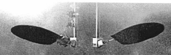
Robotic fly wings in mineral oil
Swipe sideways to see the whole figure.
Photograph of the sheet (crop of DA8.pdf): the pair of robotic wings of Dickinson's facility, which flap in a tank of mineral oil
Open the figure full size

1. Use dimensional analysis to express the lift force $F$ as a function of the minimum number of dimensionless parameters.

2. Assuming the following characteristic values for the fly: flapping frequency $f = 200$ Hz, wing length $L = 2.5$ mm, air density $\rho = 1.2$ kg/m$^3$, air viscosity $\mu = 1.8\times 10^{-5}$ kg/m·s, along with the nominal characteristics of the experiment: flapping frequency $f_e = 0.2$ Hz, wing length $L_e = 250$ mm, mineral oil density $\rho_e = 800$ kg/m$^3$, determine the mineral-oil viscosity $\mu_e$ needed to guarantee that the experiment is a physically similar representation of the fly dynamics.

3. The experimental facility including the model with $L_e = 250$ mm and the mineral oil selected above is used to investigate the variation of the lift with the flapping frequency. To that end, the wings are moved at different frequencies $f_e$ and the corresponding forces $F_e$ are measured, yielding the data points shown in the table below. Generate a curve for the variation of the force $F$ with the flapping frequency $f$ for the fly of wing length $L = 2.5$ mm.

$f_e$ (Hz)$F_e$ (N)
0.141.33
0.153.33
0.164.80
0.177.13
0.188.00
0.196.60
0.205.07
0.214.53

Source: DA8.pdf (page 1, exam of Dec 16, 2011, statement and handwritten key). Notes.pdf, Chapter 6: Π theorem, Eq. 6.25; physical similarity, Eqs. 6.57-6.59.

Worked solutionexpand / collapse

Hypotheses, Data and Dimensional Table

  • The wings have no weight and no inertia of their own, and the fly is held at a fixed point: the lift depends only on the wing motion (frequency and size, the stroke shape fixed by geometric and kinematic similarity) and on the fluid.
  • No free surface and negligible weight: no gravity.
ParameterMeaningDimensions
$F$lift (unknown)$MLT^{-2}$
$f$flapping frequency$T^{-1}$
$L$wing length$L$
$\rho$fluid density$ML^{-3}$
$\mu$fluid viscosity$ML^{-1}T^{-1}$

Application of the Π Theorem

$$ F = F(f, L, \rho, \mu) $$

$n = 4$; $(f, L, \rho)$ have independent dimensions (rows $f(0,0,-1)$, $L(1,0,0)$, $\rho(-3,1,0)$, $\det = -1\cdot(1\cdot 1 - 0\cdot(-3)) = -1 \neq 0$ expanding along the first row), so one group remains.

Force. $[F] = [\rho]^a[f]^b[L]^c$: $M:\; 1 = a$; $T:\; -2 = -b$; $L:\; 1 = -3 + c$; so $\rho f^2 L^4$.

Viscosity. $[\mu] = [\rho]^a[f]^b[L]^c$: $M:\; 1 = a$; $T:\; -1 = -b$; $L:\; -1 = -3 + c$; so $\rho f L^2$, and the group is $\rho L^2 f/\mu$, a Reynolds number with the velocity scale $fL$.

$$ \frac{F}{\rho L^4 f^2} = \Pi\left(\frac{\rho L^2 f}{\mu}\right) $$

Viscosity of the Oil

Physical similarity requires equal Reynolds numbers:

$$ \frac{\rho L^2 f}{\mu} = \frac{\rho_e L_e^2 f_e}{\mu_e} \;\Longrightarrow\; \mu_e = \mu\,\frac{\rho_e}{\rho}\left(\frac{L_e}{L}\right)^2\frac{f_e}{f} $$
$$ \mu_e = 1.8\times 10^{-5}\times\frac{800}{1.2}\times\left(\frac{250}{2.5}\right)^2\times\frac{0.2}{200} = 1.8\times 10^{-5}\times 666.7\times 10^{4}\times 10^{-3} = 0.12\ \text{kg/(m s)} $$

Lift Curve of the Fly

Each measured point, with $\mu_e = 0.12$ kg/(m s), is similar to the fly state with the same Reynolds number:

$$ \frac{\rho L^2 f}{\mu} = \frac{\rho_e L_e^2 f_e}{\mu_e} \;\Longrightarrow\; f = \frac{\rho_e}{\rho}\left(\frac{L_e}{L}\right)^2\frac{\mu}{\mu_e}\,f_e = 666.7\times 10^{4}\times 1.5\times 10^{-4}\,f_e = 1000\,f_e $$

and then equal dimensionless lift:

$$ \frac{F}{\rho L^4 f^2} = \frac{F_e}{\rho_e L_e^4 f_e^2} \;\Longrightarrow\; F = \frac{\rho}{\rho_e}\left(\frac{L}{L_e}\right)^4\left(\frac{f}{f_e}\right)^2 F_e = \frac{1.2}{800}\times 10^{-8}\times 10^{6}\,F_e = 1.5\times 10^{-5}\,F_e $$

The same factor follows in the key's form: substituting $f/f_e$ from the first relation, $F = (\rho_e/\rho)(\mu/\mu_e)^2 F_e = 666.7\times(1.5\times 10^{-4})^2 F_e = 1.5\times 10^{-5}F_e$.

$f_e$ (Hz)$F_e$ (N)$f$ (Hz)$F$ (N)
0.141.33140$2.0\times 10^{-5}$
0.153.33150$5.0\times 10^{-5}$
0.164.80160$7.2\times 10^{-5}$
0.177.13170$1.07\times 10^{-4}$
0.188.00180$1.20\times 10^{-4}$
0.196.60190$0.99\times 10^{-4}$
0.205.07200$7.6\times 10^{-5}$
0.214.53210$6.8\times 10^{-5}$

Answers and Checks

  • Reduced law: $F/(\rho L^4 f^2) = \Pi(\rho L^2 f/\mu)$.
  • Oil viscosity: $\mu_e = 0.12$ kg/(m s).
  • Fly: $f = 1000 f_e$ and $F = 1.5\times 10^{-5}F_e$; maximum lift $1.2\times 10^{-4}$ N at 180 Hz.
  • Dimensions: $\rho L^4 f^2$ is $ML^{-3}\cdot L^4\cdot T^{-2} = MLT^{-2}$, a force.
  • Order of magnitude: a fly of about 10 mg weighs $\sim 10^{-4}$ N, the order of the maximum lift, which is reasonable for a hovering insect.
  • Reynolds number of the fly: $\rho L^2 f/\mu = 1.2\times 6.25\times 10^{-6}\times 200/1.8\times 10^{-5} \simeq 83$, neither small nor large: inertia and viscosity both matter, so no limit simplifies the law and the experiment must match $\mathrm{Re}$ exactly.
  • Check against the official key: DA8.pdf gives $\mu_e = 0.12$ kg/(m s) and the table $f$ = 140 to 210 Hz with $F$ = $0.2\times 10^{-4}$, $0.5\times 10^{-4}$, $0.72\times 10^{-4}$, $1.07\times 10^{-4}$, $1.2\times 10^{-4}$, $1\times 10^{-4}$, $0.76\times 10^{-4}$, $0.68\times 10^{-4}$ N, the same values.
Problem DA9

Power of an Airplane Propeller

Original statement · DA9.pdf
Π theoremReynolds and MachStandard atmosphere

Official Problem Statement

The power $W$ needed to move the propeller of a small airplane depends on the airplane velocity $V$, propeller diameter $D$, angular velocity $\Omega$, and also on the air properties, including its density $\rho$, viscosity $\mu$, and sound velocity $c$; the latter, characterizing compressibility effects, has dimensions $[c] = LT^{-1}$. Assuming that the effect of gravity is negligible:

1. Use dimensional analysis to express the propeller power $W$ as a function of the minimum number of dimensionless parameters.

A new airplane with propeller of diameter $D = 1.5$ m is to be designed to fly at an altitude $z = 5000$ m with cruise velocity $V = 300$ Km/h and propeller angular velocity $\Omega = 2500$ rpm. To determine the needed power, an experimental model is to be tested in a wind tunnel at sea level ($z = 0$ m).

2. Determine the model diameter $D_e$, the propeller angular velocity $\Omega_e$, and the wind-tunnel velocity $V_e$ needed to guarantee that the experiment provides a physically similar representation of the airplane flight conditions.

3. For the values of $D_e$, $\Omega_e$, and $V_e$ determined above, the power measured in the experiment (obtained as the product of $\Omega_e$ and the torque acting on the propeller shaft) is $W_e = 6\times 10^7$ Watt. Obtain the power $W$ corresponding to the real airplane.

Note: Physical properties for air according to the standard atmosphere:

$z$ (m)$T$ (K)$\rho$ (kg/m$^3$)$\mu$ (kg/(m s))$c$ (m/s)
0288.151.225$1.775\times 10^{-5}$340.3
5000255.650.736$1.630\times 10^{-5}$320.5

The value $D = 1.5$ m is written by hand on the printed sheet, next to "$D$".

Source: DA9.pdf (page 1, exam of Jan 10, 2012, statement and handwritten key). Notes.pdf, Chapter 6: Π theorem, Eq. 6.25; physical similarity, Eqs. 6.57-6.59.

Worked solutionexpand / collapse

Hypotheses, Data and Dimensional Table

  • Air is a compressible gas: its compressibility enters through the speed of sound $c$ (Notes.pdf, p. 66). Gravity is negligible.
  • Prototype at $z = 5000$ m: $\rho = 0.736$ kg/m$^3$, $\mu = 1.630\times 10^{-5}$ kg/(m s), $c = 320.5$ m/s. Model at $z = 0$: $\rho_e = 1.225$ kg/m$^3$, $\mu_e = 1.775\times 10^{-5}$ kg/(m s), $c_e = 340.3$ m/s.
ParameterDimensions
$W$ (unknown)$ML^2T^{-3}$
$\rho$$ML^{-3}$
$\mu$$ML^{-1}T^{-1}$
$c$, $V$$LT^{-1}$
$D$$L$
$\Omega$$T^{-1}$

Application of the Π Theorem

$$ W = W(\rho, \mu, c, V, D, \Omega) $$

$n = 6$; $(\rho, V, D)$ have independent dimensions ($\det = -1$, as in DA1), so $n - k = 3$ groups remain.

  • Power. $[W] = [\rho][V]^3[D]^2$ (exponents as in DA1): $\Pi_0 = W/(\rho V^3 D^2)$.
  • Viscosity. $[\mu] = [\rho][V][D]$: the Reynolds number $\rho V D/\mu$.
  • Speed of sound. $[c] = [V]$: the inverse Mach number $V/c$ is the group.
  • Rotation. $[\Omega] = [V][D]^{-1}$: the group $\Omega D/V$ (the inverse of the advance ratio).
$$ \frac{W}{\rho V^3 D^2} = f\left(\frac{\rho V D}{\mu}, \frac{V}{c}, \frac{\Omega D}{V}\right) $$

Physical Similarity at Sea Level

The three groups must be equal. The Mach number fixes the tunnel speed:

$$ \frac{V}{c} = \frac{V_e}{c_e} \;\Longrightarrow\; V_e = \frac{c_e}{c}\,V = \frac{340.3}{320.5}\times 300 = 1.0618\times 300 = 318.5\ \text{km/h} \simeq 319\ \text{km/h} $$

The Reynolds number then fixes the diameter:

$$ \frac{\rho V D}{\mu} = \frac{\rho_e V_e D_e}{\mu_e} \;\Longrightarrow\; D_e = \frac{\mu_e}{\mu}\,\frac{\rho}{\rho_e}\,\frac{V}{V_e}\,D = \frac{\mu_e}{\mu}\,\frac{\rho}{\rho_e}\,\frac{c}{c_e}\,D $$
$$ D_e = \frac{1.775}{1.630}\times\frac{0.736}{1.225}\times\frac{320.5}{340.3}\times 1.5 = 1.0890\times 0.6008\times 0.9418\times 1.5 = 0.924\ \text{m} $$

The advance ratio fixes the rotation:

$$ \frac{\Omega D}{V} = \frac{\Omega_e D_e}{V_e} \;\Longrightarrow\; \Omega_e = \frac{D}{D_e}\,\frac{V_e}{V}\,\Omega = \frac{1.5}{0.924}\times 1.0618\times 2500 = 1.6229\times 1.0618\times 2500 = 4308\ \text{rpm} $$

The ratios $V/V_e$, $\Omega/\Omega_e$ are dimensionless, so km/h and rpm can be kept.

Power of the Airplane

With the three groups equal, $W/(\rho V^3 D^2)$ is equal:

$$ \frac{W}{\rho V^3 D^2} = \frac{W_e}{\rho_e V_e^3 D_e^2} \;\Longrightarrow\; W = \frac{\rho}{\rho_e}\left(\frac{V}{V_e}\right)^3\left(\frac{D}{D_e}\right)^2 W_e $$
$$ W = 0.6008\times(0.9418)^3\times(1.6229)^2\times 6\times 10^{7} = 0.6008\times 0.8354\times 2.6338\times 6\times 10^{7} = 7.93\times 10^{7}\ \text{W} $$

Answers and Checks

  • Reduced law: $W/(\rho V^3D^2) = f\left(\rho VD/\mu,\, V/c,\, \Omega D/V\right)$.
  • Model: $D_e = 0.924$ m, $V_e = 319$ km/h, $\Omega_e = 4308$ rpm.
  • Airplane power: $W = 7.9\times 10^7$ W.
  • Dimensions: as in DA1, $\rho V^3D^2$ is a power; $V/c$ and $\Omega D/V$ are pure numbers.
  • Why the model is smaller: sea-level air is denser ($\rho_e/\mu_e = 6.9\times 10^4$ s/m$^2$ against $4.5\times 10^4$ at 5000 m), so the same Reynolds number needs a smaller diameter; the faster tunnel speed (same Mach in warmer air) helps too.
  • On the data: the given $W_e = 6\times 10^7$ W is far above the real power of a small propeller (of order $10^5$ W); the conversion factor $W/W_e = 1.32$ does not depend on it.
  • Check against the official key: DA9.pdf gives $D_e = 0.924$ m, $V_e = 319$ km/h, $\Omega_e = 4308$ rpm and $W = 7.9\times 10^7$ W, the same results.
Problem DA10

Two-Belt Viscous Pump

Original statement · DA10.pdf
Π theoremRe ≪ 1Calibration table

Official Problem Statement

PROBLEM 3 (50 minutes) The system sketched in the figure is designed to steadily pump fluid of constant density $\rho$ and constant viscosity $\mu$ from a reservoir, where the modified pressure has a constant value $P_0$, to another one at pressure $P_0 + \Delta P$ ($\Delta P > 0$). To that end, a pair of parallel belts of length $L$, separated by a distance $h \ll L$, are driven at constant velocities $V_l$ and $V_u$, dragging the liquid towards the large pressure reservoir.

In the forthcoming analysis, the liquid flow can be assumed steady and two-dimensional (spanwise length much larger than $h$). The most important parameters of the system are the liquid volume flux per unit spanwise length, $q$, the power needed to drive the system per unit spanwise length, $\dot{W}$, and the pump efficiency, $\eta = q\Delta P/\dot{W}$.

Vu Vl h L P0 P0 + ΔP ρ, μ
Swipe sideways to see the whole figure.
Statement figure (redrawn from DA10.pdf): two parallel belts of length L, a distance h ≪ L apart, driven at V_u and V_l, drag liquid of density ρ and viscosity μ from a reservoir at reduced pressure P_0 to one at P_0 + ΔP
Open the figure full size

1. (*3 points*). Use dimensional analysis to simplify the dependence of $q$, $\dot{W}$ and $\eta$, as functions of an appropriately chosen set of parameters governing the operation of the pump.

2. (*2 points*). Simplify the resulting dimensionless functions when the inertia of the fluid can be neglected compared to the viscous forces. Note that, in this limit, the fluid density plays a negligible role. In the remainder of the problem, assume that these conditions are satisfied.

A pump with $h = 1$ cm and $L = 20$ cm is calibrated using glycerol, of density $\rho_g = 1260$ kg/m$^3$ and viscosity $\mu_g = 1.41$ kg/(m s), using an overpressure $\Delta P_g = 1$ kPa. During the calibration process, the lower belt is kept at rest, $V_{l,g} = 0$, while the upper belt is driven at several velocities $V_{u,g}$, as indicated in the table below, where the corresponding values of $q_g$, $\dot{W}_g$ and $\eta_g$ are also shown.

$V_{u,g}$ (cm/s)$q_g$ (cm$^2$/s)$\dot{W}_g$ (Watt/m)$\eta_g$
1020.80.26
154.51.40.33
2072.10.33
259.530.32
301240.3
3514.55.20.28

The same pump is used to deliver a silicone oil, of density $\rho_{oil} = 1100$ kg m$^{-3}$ and viscosity $\mu_{oil} = 5$ kg/(m s), with an overpressure $\Delta P_{oil} = 2$ kPa.

3. (*2 points*). Determine the velocities $V_{l,oil}$ and $V_{u,oil}$ for which the results obtained in the calibration tests can be used to predict the pumping behavior with the silicone oil.

4. (*2 points*). Calculate the corresponding values of $q_{oil}$, $\dot{W}_{oil}$ and $\eta_{oil}$.

5. (*1 point*). Discuss the hypothesis of negligible fluid inertia.

Source: DA10.pdf (page 1: statement; page 2: handwritten key). Notes.pdf, Chapter 6: Π theorem, Eq. 6.25; selection of parameters, p. 68; limits, Eq. 6.55; physical similarity, Eqs. 6.57-6.59.

Worked solutionexpand / collapse

Hypotheses, Data and Dimensional Table

  • Steady, two-dimensional flow of a liquid with constant $\rho$ and $\mu$; gravity is absorbed in the modified pressure, so only the difference $\Delta P$ enters (Notes.pdf, p. 66).
  • All quantities are per unit spanwise length: $[q] = L^2T^{-1}$, $[\dot{W}] = ML^2T^{-3}/L = MLT^{-3}$.
  • Recomputing $\eta = q\Delta P/\dot{W}$ from the table: row 1 gives $2\times 10^{-4}\times 10^{3}/0.8 = 0.25$ (printed 0.26) and row 2 gives $4.5\times 10^{-4}\times 10^{3}/1.4 = 0.32$ (printed 0.33); rows 3 to 6 agree with the printed values (0.333, 0.317, 0.300, 0.279).
ParameterDimensions
$q$$L^2T^{-1}$
$\dot{W}$$MLT^{-3}$
$\eta$1
$\rho$$ML^{-3}$
$\mu$$ML^{-1}T^{-1}$
$\Delta P$$ML^{-1}T^{-2}$
$V_u$, $V_l$$LT^{-1}$
$L$, $h$$L$

Application of the Π Theorem

$$ q = f_1(\rho, \mu, \Delta P, V_u, V_l, L, h), \qquad \dot{W} = f_2(\dots), \qquad \eta = f_3(\dots) $$

$n = 7$. The key takes $(\mu, V_u, h)$, natural for a viscous pump. Rows $\mu(-1, 1, -1)$, $V_u(1, 0, -1)$, $h(1, 0, 0)$ in $(L, M, T)$; only $\mu$ has mass, so expanding along the $M$ column, $\det = -1\cdot\left(1\cdot 0 - (-1)\cdot 1\right) = -1 \neq 0$: $k = 3$, and $n - k = 4$ groups remain.

Flux. $[q] = [\mu]^a[V_u]^b[h]^c$: $M:\; 0 = a$; $T:\; -1 = -b$; $L:\; 2 = b + c$; so the scale is $V_u h$.

Power. $[\dot{W}] = [\mu]^a[V_u]^b[h]^c$: $M:\; 1 = a$; $T:\; -3 = -a - b$, $b = 2$; $L:\; 1 = -a + b + c$, $c = 0$; so the scale is $\mu V_u^2$.

Density. $[\rho] = [\mu]^a[V_u]^b[h]^c$: $M:\; 1 = a$; $T:\; 0 = -1 - b$, $b = -1$; $L:\; -3 = -1 - 1 + c$, $c = -1$: the group $\rho V_u h/\mu$, a Reynolds number.

Pressure. $[\Delta P] = [\mu]^a[V_u]^b[h]^c$: $M:\; 1 = a$; $T:\; -2 = -1 - b$, $b = 1$; $L:\; -1 = -1 + 1 + c$, $c = -1$: the group $h\Delta P/(\mu V_u)$.

Belts and geometry. $V_l/V_u$ and $L/h$.

$$ \frac{q}{V_u h} = \Pi_q\left(\frac{\rho V_u h}{\mu}, \frac{h\Delta P}{\mu V_u}, \frac{V_l}{V_u}, \frac{L}{h}\right), \quad \frac{\dot{W}}{\mu V_u^2} = \Pi_W(\dots), \quad \eta = \eta(\dots) $$

with the same four arguments.

Negligible Inertia

When inertia is negligible against viscous forces, the density drops out ($\rho V_u h/\mu \to 0$; Notes.pdf, Eq. 6.55):

$$ \frac{q}{V_u h} = \Pi_q\left(\frac{h\Delta P}{\mu V_u}, \frac{V_l}{V_u}, \frac{L}{h}\right), \quad \frac{\dot{W}}{\mu V_u^2} = \Pi_W\left(\frac{h\Delta P}{\mu V_u}, \frac{V_l}{V_u}, \frac{L}{h}\right), \quad \eta = \eta\left(\frac{h\Delta P}{\mu V_u}, \frac{V_l}{V_u}, \frac{L}{h}\right) $$

Physical Similarity: from Glycerol to Silicone Oil

The pump is the same, so $L/h$ is the same. The other two groups must be equal.

Lower belt.

$$ \frac{V_{l,oil}}{V_{u,oil}} = \frac{V_{l,g}}{V_{u,g}} = 0 \;\Longrightarrow\; V_{l,oil} = 0 $$

Upper belt. The same $h$ cancels:

$$ \frac{h\Delta P_{oil}}{\mu_{oil}V_{u,oil}} = \frac{h\Delta P_g}{\mu_g V_{u,g}} \;\Longrightarrow\; \frac{V_{u,oil}}{V_{u,g}} = \frac{\mu_g}{\mu_{oil}}\,\frac{\Delta P_{oil}}{\Delta P_g} = \frac{1.41}{5}\times\frac{2}{1} = 0.564 $$

Oil Performance

With all groups equal, the dimensionless outputs are equal:

$$ \frac{q_{oil}}{V_{u,oil}h} = \frac{q_g}{V_{u,g}h} \;\Longrightarrow\; \frac{q_{oil}}{q_g} = \frac{V_{u,oil}}{V_{u,g}} = 0.564 $$
$$ \frac{\dot{W}_{oil}}{\mu_{oil}V_{u,oil}^2} = \frac{\dot{W}_g}{\mu_g V_{u,g}^2} \;\Longrightarrow\; \frac{\dot{W}_{oil}}{\dot{W}_g} = \frac{\mu_{oil}}{\mu_g}\left(\frac{V_{u,oil}}{V_{u,g}}\right)^2 = \frac{5}{1.41}\times 0.564^2 = 3.546\times 0.3181 = 1.128 $$
$$ \eta_{oil} = \eta_g $$

Check: $\eta_{oil}/\eta_g = (q_{oil}/q_g)(\Delta P_{oil}/\Delta P_g)/(\dot{W}_{oil}/\dot{W}_g) = 0.564\times 2/1.128 = 1$. The $\eta_{oil}$ column copies the printed $\eta_g$, as the key does; from $q\Delta P/\dot{W}$ the first two rows would read 0.25 and 0.32.

$V_{u,g}$ (cm/s)$V_{u,oil}$ (cm/s)$q_{oil}$ (cm$^2$/s)$\dot{W}_{oil}$ (W/m)$\eta_{oil}$
105.641.1280.9020.26
158.462.5381.5790.33
2011.283.9482.3690.33
2514.105.3583.3840.32
3016.926.7684.5120.30
3519.748.1785.8660.28

Negligible Inertia: Discussion

The plain Reynolds number of the calibration is not small: $\rho_g V_{u,g}h/\mu_g = 1260\times 0.10\times 0.01/1.41 = 0.89$ at the lowest speed and $3.1$ at the highest. The key compares inertia and viscosity in the slender channel ($h \ll L$), where the convective term is smaller than the viscous one by the extra factor $h/L$, so the relevant number is the reduced Reynolds number $(\rho V_u h/\mu)(h/L)$. This criterion belongs to the slender viscous flows of Chapter 7 of the notes (an extension here). With $h/L = 1/20$:

$$ \text{glycerol: } 0.89\times\frac{1}{20} = 0.045 \;\le\; \frac{\rho_g V_{u,g}h}{\mu_g}\,\frac{h}{L} \;\le\; 3.13\times\frac{1}{20} = 0.156 $$
$$ \text{oil: } \frac{1100\times 0.0564\times 0.01}{5}\times\frac{1}{20} = 0.0062 \;\le\; \frac{\rho_{oil}V_{u,oil}h}{\mu_{oil}}\,\frac{h}{L} \;\le\; \frac{1100\times 0.1974\times 0.01}{5}\times\frac{1}{20} = 0.022 $$

Both are small, more so for the oil, so neglecting inertia is a good approximation, and the calibration can be transferred to the oil.

Answers and Checks

  • Reduced laws: $q/(V_uh)$, $\dot{W}/(\mu V_u^2)$ and $\eta$ are functions of $\rho V_uh/\mu$, $h\Delta P/(\mu V_u)$, $V_l/V_u$, $L/h$; without inertia, of the last three only.
  • Similar operation with oil: $V_{l,oil} = 0$, $V_{u,oil} = 0.564\,V_{u,g}$.
  • Oil performance: $q_{oil} = 0.564\,q_g$, $\dot{W}_{oil} = 1.128\,\dot{W}_g$, $\eta_{oil} = \eta_g$ (table above).
  • Inertia: reduced Reynolds number 0.045-0.156 (glycerol) and 0.006-0.022 (oil).
  • Dimensions: $\mu V_u^2$ is $ML^{-1}T^{-1}\cdot L^2T^{-2} = MLT^{-3}$, a power per unit length; $h\Delta P/(\mu V_u)$ is $L\cdot ML^{-1}T^{-2}/(ML^{-1}T^{-1}\cdot LT^{-1}) = 1$.
  • Check against the official key: DA10.pdf gives $V_{l,oil} = 0$, $V_{u,oil}/V_{u,g} = 0.564$, $q_{oil}/q_g = 0.564$, $\dot{W}_{oil}/\dot{W}_g = 1.128$ and the same table, with the inertia ranges 0.045-0.156 and 0.0062-0.022.
Problem DA11

Power of a Wave Generator

Original statement · DA11.pdf
Π theoremFroude similarityRe ≫ 1

Official Problem Statement

PROBLEM 3 (45 minutes) The figure below illustrates a simple mechanism to generate periodic gravity waves in a pool of liquid (density $\rho$ and viscosity $\mu$), with undisturbed height $H$. The waves are driven by the harmonic motion of the lateral confining wall perpendicular to itself, with amplitude $A$ and frequency $\omega$.

H ρ, μ g x = A cos(2πωt) V Ẇ
Swipe sideways to see the whole figure.
Statement figure (redrawn from DA11.pdf): above, the pool of liquid (ρ, μ) of undisturbed depth H; below, the lateral wall moved harmonically, x = A cos(2πωt), by the power Ẇ, generating gravity waves
Open the figure full size

1. (*4 points*). Use dimensional analysis to simplify the dependence of the power needed to drive the generator, $\dot{W}$, as a function of the governing parameters $(\rho, \mu, A, \omega, H, g)$.

2. (*1 point*). Simplify the resulting dimensionless function for the case of negligible viscous forces. In the remainder of the problem, assume that this condition is satisfied.

To characterize the requirements of a new wave generator to be installed in a large water channel (subindex p), a scale model (subindex m) with $H_m/H_p = 1/20$ is tested in the lab using water as working fluid. Knowing that the wave frequency required in the water channel is $\omega_p = 1/6$ s$^{-1}$,

3. (*2 points*). Determine the value of the frequency, $\omega_m$, that must be used in the experiments to guarantee physical similarity.

4. (*2 points*). If the power used in the model is $\dot{W}_m = 1$ Watt, obtain the power needed to drive the wave generator in the water channel, $\dot{W}_p$.

5. (*1 point*). Justify the hypothesis of negligible viscous forces. If needed, make a reasonable guess for the values of the involved variables.

Source: DA11.pdf (page 1: statement; page 2: handwritten key). Notes.pdf, Chapter 6: Π theorem, Eq. 6.25; limits, Eq. 6.55; physical similarity, Eqs. 6.57-6.59.

Worked solutionexpand / collapse

Hypotheses, Data and Dimensional Table

  • Gravity waves at a free surface: $g$ is essential (Notes.pdf, p. 66). The wall motion $x = A\cos(2\pi\omega t)$ shows that $\omega$ is a frequency in cycles per second, $[\omega] = T^{-1}$.
  • The model is geometrically similar (all lengths, the channel width included, scaled by $1/20$) and uses water, as the channel: same $\rho$, $\mu$, $g$.
ParameterDimensions
$\dot{W}$ (unknown)$ML^2T^{-3}$
$\rho$$ML^{-3}$
$\mu$$ML^{-1}T^{-1}$
$A$, $H$$L$
$\omega$$T^{-1}$
$g$$LT^{-2}$

Application of the Π Theorem

$$ \dot{W} = f(\rho, \mu, A, \omega, H, g) $$

$n = 6$. The key takes $(\rho, A, \omega)$: rows $\rho(-3, 1, 0)$, $A(1, 0, 0)$, $\omega(0, 0, -1)$ in $(L, M, T)$; expanding along the $\omega$ row, $\det = (-1)\cdot\left((-3)\cdot 0 - 1\cdot 1\right) = 1 \neq 0$, so $k = 3$ and three groups remain.

Power. $[\dot{W}] = [\rho]^a[\omega]^b[A]^c$: $M:\; 1 = a$; $T:\; -3 = -b$; $L:\; 2 = -3 + c$; so $\Pi_{\dot{W}} = \dot{W}/(\rho\omega^3A^5)$.

Viscosity. $[\mu] = [\rho]^a[\omega]^b[A]^c$: $M:\; 1 = a$; $T:\; -1 = -b$; $L:\; -1 = -3 + c$; so $\Pi_\mu = \mu/(\rho\omega A^2)$, the inverse of a Reynolds number with the wall velocity $\omega A$.

Depth. $\Pi_H = H/A$.

Gravity. $[g] = [\omega]^b[A]^c$: $T:\; -2 = -b$; $L:\; 1 = c$; so $\Pi_g = g/(\omega^2A)$.

$$ \Pi_{\dot{W}} = \Pi_{\dot{W}}(\Pi_\mu, \Pi_H, \Pi_g): \qquad \frac{\dot{W}}{\rho\omega^3A^5} = \Pi_{\dot{W}}\left(\frac{\mu}{\rho\omega A^2}, \frac{H}{A}, \frac{g}{\omega^2 A}\right) $$

Negligible Viscous Forces

For $\Pi_\mu \to 0$ the group drops out (Notes.pdf, Eq. 6.55):

$$ \frac{\dot{W}}{\rho\omega^3A^5} = \Pi_{\dot{W}}\left(\frac{H}{A}, \frac{g}{\omega^2 A}\right) $$

Physical Similarity

Depth group. Geometric similarity of the whole setup, amplitude included:

$$ \frac{H_p}{A_p} = \frac{H_m}{A_m} \;\Longrightarrow\; \frac{A_p}{A_m} = \frac{H_p}{H_m} = 20 $$

Gravity group. Same $g$:

$$ \frac{g}{\omega_p^2A_p} = \frac{g}{\omega_m^2A_m} \;\Longrightarrow\; \frac{\omega_m}{\omega_p} = \sqrt{\frac{A_p}{A_m}} = \sqrt{20} $$
$$ \omega_m = \sqrt{20}\times\frac{1}{6} = \frac{2\sqrt{5}}{6} = \frac{\sqrt{5}}{3}\ \text{s}^{-1} = 0.745\ \text{s}^{-1} $$

Power of the Prototype

With $\Pi_H$ and $\Pi_g$ equal, $\Pi_{\dot{W}}$ is equal (same $\rho$):

$$ \frac{\dot{W}_p}{\rho\omega_p^3A_p^5} = \frac{\dot{W}_m}{\rho\omega_m^3A_m^5} \;\Longrightarrow\; \frac{\dot{W}_p}{\dot{W}_m} = \left(\frac{\omega_p}{\omega_m}\right)^3\left(\frac{A_p}{A_m}\right)^5 = \left(\frac{A_p}{A_m}\right)^{-3/2}\left(\frac{A_p}{A_m}\right)^5 = \left(\frac{A_p}{A_m}\right)^{7/2} $$
$$ \dot{W}_p = 20^{7/2}\times 1\ \text{W} = 20^3\times\sqrt{20}\ \text{W} = 8000\times 4.472 = 35\,777\ \text{W} = 35.78\ \text{kW} $$

Negligible Viscosity: Justification

For water, $\rho = 10^3$ kg/m$^3$ and $\mu = 10^{-3}$ kg/(m s), so $\Pi_\mu = 10^{-6}/(\omega A^2)$ with $\omega$ in s$^{-1}$ and $A$ in m. The amplitudes are not given; reasonable guesses, as the key suggests:

  • channel: $A_p \sim 1$ m, $\omega_p = 1/6$ s$^{-1}$, so $\Pi_\mu \sim 10^{-6}/(0.17\times 1) = 6\times 10^{-6} \ll 1$;
  • model: $A_m = A_p/20 \sim 0.05$ m, $\omega_m = 0.745$ s$^{-1}$, so $\Pi_\mu \sim 10^{-6}/(0.745\times 0.0025) = 5\times 10^{-4} \ll 1$.

Viscous forces are negligible in both (large Reynolds numbers).

Answers and Checks

  • Reduced law: $\dot{W}/(\rho\omega^3A^5) = \Pi_{\dot{W}}\left(\mu/(\rho\omega A^2),\, H/A,\, g/(\omega^2A)\right)$; without viscosity, $\Pi_{\dot{W}}(H/A, g/(\omega^2A))$.
  • Model frequency: $\omega_m = \sqrt{5}/3 = 0.745$ s$^{-1}$.
  • Channel power: $\dot{W}_p = 20^{7/2}\,\dot{W}_m = 35.78$ kW.
  • Dimensions: $\rho\omega^3A^5$ is $ML^{-3}\cdot T^{-3}\cdot L^5 = ML^2T^{-3}$, a power.
  • Froude scaling: times scale as $\lambda^{1/2}$ and powers as $\lambda^{7/2}$ with $\lambda = 20$, as for the ship of DA1.
  • Check against the official key: DA11.pdf gives $\omega_m = \sqrt{5}/3$ s$^{-1}$ and $\dot{W}_p = 20^{7/2}\dot{W}_m = 35.78$ kW, and justifies $\Pi_\mu \ll 1$ with $A \sim 1$ m, $\omega \sim 1$ s$^{-1}$.
Problem DA12

Supersonic Missile Drag and Shock Standoff

Original statement · DA12.pdf
Π theoremMach similarityOrder of magnitudeHypersonic limit

Official Problem Statement

A nuclear missile is designed to fly at supersonic speeds (velocities $U$ larger than the sound velocity $c$) at high altitudes. In the solution that appears, a bow shock is present at a standoff distance $d$ from the missile tip. To characterize the solution and determine the drag force $F$ acting on the missile, a series of experiments is conducted in a supersonic wind tunnel using a small experimental model geometrically similar to the real prototype. Analyze the results following these steps:

1. Use the Π theorem to reduce the parametric dependence of the drag $F$ and standoff distance $d$. To set up the problem, note that the compressibility of the gas is characterized by the ambient sound speed $c$, which should be considered at the start of the analysis, along with the ambient values of the density and viscosity of the gas $\rho$ and $\mu$. Since the density changes across the shock, gravity might also influence the solution through the resulting buoyant force.

2. Derive the conditions under which both gravity and viscosity do not influence the solution. The reasoning should be substantiated with an order-of-magnitude analysis of the momentum equation to show clearly which dimensionless parameters measure the relative importance of buoyant and viscous forces (relative to the convective acceleration).

3. The experimental tests are carried out at normal ambient conditions ($\rho_e = 1.22$ kg/m$^3$, $\mu_e = 1.98\times 10^{-5}$ kg/(m s), $c_e = 340$ m/s) with a model of diameter $D_e = 0.01$ m, significantly smaller than that of the real missile ($D_m = 1$ m), giving the results shown in the table. Use the results, together with the assumption that $g$ and $\mu$ have a negligible influence, to deduce the variation with flight speed $U_m$ of the drag force $F_m$ and standoff distance $d_m$ corresponding to the missile flying at cruise altitude, where $\rho_m = 0.36$ kg/m$^3$, $\mu_m = 1.44\times 10^{-5}$ kg/(m s), and $c_m = 295$ m/s.

4. Check that the criteria needed to neglect $g$ and $\mu$ are satisfied both in the experiment and for the real missile conditions.

5. Determine a simplified expression for the drag force when the Mach number is very large (i.e., $U/c \gg 1$).

$U_e$ (m/s)$F_e$ (N)$d_e$ (m)
4009.20.012
70037.500.01
1,00086.000.005
2,0003830
4,00015320
D bow shock d U ρ, μ c g
Swipe sideways to see the whole figure.
Statement figure (redrawn from DA12.pdf, frame of the missile): a gas of density ρ, viscosity μ and sound speed c meets the missile of diameter D at a speed U > c; a bow shock stands at a distance d ahead of the tip
Open the figure full size

Source: DA12.pdf (page 1, prefinal exam of Dec 16, 2013, statement and handwritten key). Notes.pdf, Chapter 6: Π theorem, Eq. 6.25; order of magnitude, Eqs. 6.45-6.46; limits, Eq. 6.55; physical similarity, Eqs. 6.57-6.59.

Worked solutionexpand / collapse

Hypotheses, Data and Dimensional Table

  • In the frame of the missile the gas arrives at $U$ with its ambient $\rho$, $\mu$, $c$; gravity is kept at first, as the statement asks, because the density jump across the shock creates a buoyant force.
  • The model is geometrically similar; the subscript $m$ is the missile (prototype), $e$ the experiment.
ParameterDimensions
$F$ (unknown)$MLT^{-2}$
$d$ (unknown)$L$
$D$$L$
$U$, $c$$LT^{-1}$
$\rho$$ML^{-3}$
$\mu$$ML^{-1}T^{-1}$
$g$$LT^{-2}$

Application of the Π Theorem

$$ F = F(D, U, \rho, \mu, c, g), \qquad d = d(D, U, \rho, \mu, c, g) $$

$n = 6$; $(\rho, U, D)$ have independent dimensions ($\det = -1$, as in DA1), so three groups remain.

  • Drag: $[F] = [\rho][U]^2[D]^2$ (exponents as for the sphere, Notes.pdf, Eq. 6.32): $F/(\rho U^2D^2)$.
  • Standoff: $d/D$.
  • Viscosity: $\rho UD/\mu$ (Reynolds). Gravity: $[g] = [U]^2[D]^{-1}$ (as in DA1): $U^2/(gD)$ (Froude squared). Compressibility: $U/c$ (Mach).
$$ \frac{F}{\rho U^2D^2} = f_1\left(\frac{\rho UD}{\mu}, \frac{U^2}{gD}, \frac{U}{c}\right), \qquad \frac{d}{D} = f_2\left(\frac{\rho UD}{\mu}, \frac{U^2}{gD}, \frac{U}{c}\right) $$

Order of Magnitude: When Gravity and Viscosity Do Not Matter

Velocities are of order $U$ and change by $O(U)$ over distances $O(D)$, as in Notes.pdf, Eq. 6.45. The convective acceleration, the viscous force and the buoyant force per unit volume are then

$$ O(\rho\,\bar{v}\cdot\nabla\bar{v}) \sim \frac{\rho U^2}{D}, \qquad O(\mu\nabla^2\bar{v}) \sim \frac{\mu U}{D^2}, \qquad O(\Delta\rho\,g) \sim \rho g $$

where the density change across a strong shock is of the order of $\rho$ itself. The two ratios to the convective term are

$$ \frac{O(\rho\,\bar{v}\cdot\nabla\bar{v})}{O(\mu\nabla^2\bar{v})} = \frac{\rho U^2/D}{\mu U/D^2} = \frac{\rho UD}{\mu}, \qquad \frac{O(\rho\,\bar{v}\cdot\nabla\bar{v})}{O(\rho g)} = \frac{\rho U^2/D}{\rho g} = \frac{U^2}{gD} $$

So viscosity is negligible if $\rho UD/\mu \gg 1$, and gravity if $U^2/(gD) \gg 1$. Then (Notes.pdf, Eq. 6.55)

$$ \frac{F}{\rho U^2D^2} = f_1\left(\frac{U}{c}\right), \qquad \frac{d}{D} = f_2\left(\frac{U}{c}\right) $$

Mach Similarity: from the Tunnel to the Missile

Each tunnel point is similar to the flight state with the same Mach number:

$$ \frac{U_m}{c_m} = \frac{U_e}{c_e} \;\Longrightarrow\; U_m = \frac{c_m}{c_e}\,U_e = \frac{295}{340}\,U_e = 0.8676\,U_e $$

and then

$$ \frac{F_m}{\rho_mU_m^2D_m^2} = \frac{F_e}{\rho_eU_e^2D_e^2} \;\Longrightarrow\; F_m = \frac{\rho_m}{\rho_e}\left(\frac{U_m}{U_e}\right)^2\left(\frac{D_m}{D_e}\right)^2F_e = \frac{0.36}{1.22}\times 0.7528\times 10^{4}\,F_e = 2221\,F_e $$
$$ \frac{d_m}{D_m} = \frac{d_e}{D_e} \;\Longrightarrow\; d_m = \frac{D_m}{D_e}\,d_e = 100\,d_e $$
$U_e$ (m/s)$U_m$ (m/s)$F_m$ (N)$d_m$ (m)
400347$2.04\times 10^{4}$1.2
700607$8.33\times 10^{4}$1.0
1000868$1.91\times 10^{5}$0.5
20001735$8.51\times 10^{5}$0
40003471$3.40\times 10^{6}$0
Discrepancy with the official solution

The key writes $F_m = 1.91\times 10^{4}$ N in the third row; $2221\times 86 = 1.91\times 10^{5}$ N, and the drag must grow between the second row ($8.33\times 10^{4}$ N) and the fourth ($8.5\times 10^{5}$ N), so the exponent of the key is a slip: the value is $1.91\times 10^{5}$ N.

Check of the Criteria

The groups are smallest at the lowest speed of each series:

$$ \left(\frac{\rho_eU_eD_e}{\mu_e}\right)_{min} = \frac{1.22\times 400\times 0.01}{1.98\times 10^{-5}} = 2.46\times 10^{5} \gg 1, \qquad \left(\frac{\rho_mU_mD_m}{\mu_m}\right)_{min} = \frac{0.36\times 347\times 1}{1.44\times 10^{-5}} = 8.68\times 10^{6} \gg 1 $$
$$ \left(\frac{U_e^2}{gD_e}\right)_{min} = \frac{400^2}{9.81\times 0.01} = 1.63\times 10^{6} \gg 1, \qquad \left(\frac{U_m^2}{gD_m}\right)_{min} = \frac{347^2}{9.81\times 1} = 1.23\times 10^{4} \gg 1 $$

All four are very large: gravity and viscosity can be neglected in the tunnel and in flight.

Hypersonic Limit

For $U/c \gg 1$ the Mach number stops influencing the drag coefficient (Notes.pdf, Eq. 6.55):

$$ \frac{F}{\rho U^2D^2} = C $$

The tunnel data give $C$:

$U_e/c_e$$F_e/(\rho_eU_e^2D_e^2)$
1.18$9.2/(1.22\times 1.6\times 10^{5}\times 10^{-4}) = 0.471$
2.06$37.5/(1.22\times 4.9\times 10^{5}\times 10^{-4}) = 0.627$
2.94$86/(1.22\times 10^{6}\times 10^{-4}) = 0.705$
5.88$383/(1.22\times 4\times 10^{6}\times 10^{-4}) = 0.785$
11.8$1532/(1.22\times 1.6\times 10^{7}\times 10^{-4}) = 0.785$

The last two Mach numbers give the same value, so $C \simeq 0.785$ and

$$ F \simeq 0.785\,\rho U^2D^2 \qquad (U/c \gg 1) $$

Answers and Checks

  • Reduced laws: $F/(\rho U^2D^2)$ and $d/D$ are functions of $\rho UD/\mu$, $U^2/(gD)$ and $U/c$.
  • Viscosity and gravity are negligible for $\rho UD/\mu \gg 1$ and $U^2/(gD) \gg 1$; then both depend on $U/c$ only.
  • Missile: $U_m = 0.868\,U_e$, $F_m = 2221\,F_e$, $d_m = 100\,d_e$ (table above).
  • Criteria: Reynolds $\ge 2.4\times 10^5$ and Froude squared $\ge 1.2\times 10^4$ in both systems.
  • Hypersonic drag: $F \simeq 0.785\,\rho U^2D^2$.
  • Dimensions: $\rho U^2D^2$ is $ML^{-3}\cdot L^2T^{-2}\cdot L^2 = MLT^{-2}$, a force.
  • Physical sense: as the Mach number grows the shock moves closer to the tip ($d \to 0$ from $U_e = 2000$ m/s on) and the drag coefficient levels off, the behaviour predicted by (6.55).
  • Check against the official key: DA12.pdf gives the same groups, $U_m = (c_m/c_e)U_e$, the same table (with the slip of the third force corrected above), the criteria $2.46\times 10^5$, $8.67\times 10^6$, $1.63\times 10^6$, $1.23\times 10^4$ and $C \simeq 0.785$.
Problem DA13

Mars Lander Parachute

Original statement · DA13.pdf
Π theoremFroude similarityDifferent planet

Official Problem Statement

Problem 3: We want to deposit a module of mass $m$ over the surface of Mars ($\mu_M = 1.2\times 10^{-5}$ kg/(m s), $\rho_M = 0.02$ kg/m$^3$, and $g_M = 3.73$ m/s$^2$) using a parachute of diameter $D_M = 5$ m. To assess the potential damage on landing, we need to know the terminal velocity of parachute descent over Mars $V_M$. For its determination, a series of experiments is carried out in a vertical wind tunnel on Earth ($\mu_E = 1.7\times 10^{-5}$ kg/(m s), $\rho_E = 1.2$ kg/m$^3$, and $g_E = 9.81$ m/s$^2$), using the mission module attached to a model parachute, geometrically similar to that to be used in the Mars mission, but with a different diameter $D_E$. Use dimensional analysis to guide the design of the experiment and the analysis of the results, following the steps given below:

1. Use the Π theorem to express the dependence of $V$ in terms of the minimum number of parameters.

2. Indicate the condition that needs to be satisfied for the effect of viscosity to be negligible. Adopt this simplification in the following.

3. Determine the diameter $D_E$ needed to maintain physical similarity.

4. A terminal velocity $V_E = 2$ m/s is measured in the wind tunnel. Obtain the terminal velocity expected in the Mars mission $V_M$.

5. Verify that the viscosity is actually negligible for the experimental and mission conditions.

m D g V
Swipe sideways to see the whole figure.
Statement figure (redrawn from DA13.pdf): a module of mass m hangs from a parachute of diameter D and falls at its terminal velocity V under gravity g
Open the figure full size

Source: DA13.pdf (page 1, final exam of Jan 21, 2014, statement and handwritten key). Notes.pdf, Chapter 6: Π theorem, Eq. 6.25; limits, Eq. 6.55; physical similarity, Eqs. 6.57-6.59.

Worked solutionexpand / collapse

Hypotheses, Data and Dimensional Table

  • At terminal velocity the weight $mg$ balances the aerodynamic drag of parachute and module; the parachute shape is fixed by geometric similarity, so it is described by $D$.
  • The same module is used in the tunnel: $m$ is the same in both systems.
  • The gas is treated as incompressible (descent speeds of a few m/s).
ParameterMeaningDimensions
$V$terminal velocity (unknown)$LT^{-1}$
$\rho$atmosphere density$ML^{-3}$
$\mu$atmosphere viscosity$ML^{-1}T^{-1}$
$g$gravity$LT^{-2}$
$m$module mass$M$
$D$parachute diameter$L$

Application of the Π Theorem

$$ V = V(\rho, \mu, g, m, D) $$

$n = 5$; the key takes $(\rho, g, D)$, with $\det = 2 \neq 0$ (rows $D(1,0,0)$, $g(1,0,-2)$, $\rho(-3,1,0)$, as in DA4), so $k = 3$ and two groups remain. The exponents are those of DA4 with $D$ in place of the particle diameter:

  • Velocity: $\sqrt{gD}$, a Froude number $V/\sqrt{gD}$.
  • Viscosity: $\mu/(g^{1/2}D^{3/2}\rho)$.
  • Mass: $m/(\rho D^3)$, the module mass against the mass of air in a volume $D^3$.
$$ \frac{V}{\sqrt{gD}} = f\left(\frac{\mu}{g^{1/2}D^{3/2}\rho}, \frac{m}{\rho D^3}\right) $$

Negligible Viscosity

The viscosity group is the inverse of a Reynolds number built with $\sqrt{gD}$; equivalently, viscosity is negligible when the Reynolds number of the descent is large,

$$ \frac{\rho VD}{\mu} \gg 1 $$

and then (Notes.pdf, Eq. 6.55)

$$ \frac{V}{\sqrt{gD}} = f\left(\frac{m}{\rho D^3}\right) $$

Diameter of the Model Parachute

Only $m/(\rho D^3)$ must be matched, with the same $m$:

$$ \frac{m}{\rho_E D_E^3} = \frac{m}{\rho_M D_M^3} \;\Longrightarrow\; D_E = D_M\left(\frac{\rho_M}{\rho_E}\right)^{1/3} = 5\times\left(\frac{0.02}{1.2}\right)^{1/3} = 5\times 0.2554 = 1.28\ \text{m} $$

The thin Martian air needs a parachute $(\rho_E/\rho_M)^{1/3} = 60^{1/3} = 3.9$ times wider than on Earth for the same module.

Terminal Velocity on Mars

With $m/(\rho D^3)$ equal, the Froude numbers are equal:

$$ \frac{V_E}{\sqrt{g_ED_E}} = \frac{V_M}{\sqrt{g_MD_M}} \;\Longrightarrow\; V_M = \sqrt{\frac{g_MD_M}{g_ED_E}}\,V_E = \left(\frac{g_M}{g_E}\right)^{1/2}\left(\frac{\rho_E}{\rho_M}\right)^{1/6}V_E $$

using $D_M/D_E = (\rho_E/\rho_M)^{1/3}$, whose square root is $(\rho_E/\rho_M)^{1/6}$. Numbers: $(3.73/9.81)^{1/2} = 0.3802^{1/2} = 0.6166$ and $60^{1/6} = 1.979$:

$$ V_M = 0.6166\times 1.979\times 2 = 2.44\ \text{m/s} $$

Check of Negligible Viscosity

$$ \text{Earth: } \frac{\rho_EV_ED_E}{\mu_E} = \frac{1.2\times 2\times 1.28}{1.7\times 10^{-5}} = 1.81\times 10^{5} \gg 1, \qquad \text{Mars: } \frac{\rho_MV_MD_M}{\mu_M} = \frac{0.02\times 2.44\times 5}{1.2\times 10^{-5}} = 2.03\times 10^{4} \gg 1 $$

Viscosity is negligible in both.

Answers and Checks

  • Reduced law: $V/\sqrt{gD} = f\left(\mu/(g^{1/2}D^{3/2}\rho),\, m/(\rho D^3)\right)$.
  • Viscosity negligible if $\rho VD/\mu \gg 1$; then $V/\sqrt{gD} = f\left(m/(\rho D^3)\right)$.
  • Model parachute: $D_E = 1.28$ m.
  • Mars terminal velocity: $V_M = 2.44$ m/s.
  • Reynolds numbers: $1.8\times 10^5$ (Earth) and $2.0\times 10^4$ (Mars).
  • Dimensions: $\sqrt{gD}$ is $(LT^{-2}\cdot L)^{1/2} = LT^{-1}$; $m/(\rho D^3)$ is $M/(ML^{-3}L^3) = 1$.
  • Physical check: in the limit $\mathrm{Re}\gg 1$ the drag is $\propto \rho V^2D^2$ (Notes.pdf, Eq. 6.51), and the balance $mg \propto \rho V^2D^2$ gives $V \propto (mg/\rho)^{1/2}/D$; with $\rho D^3$ fixed, $V_M/V_E = (g_M/g_E)^{1/2}(\rho_E/\rho_M)^{1/2}(D_E/D_M) = 0.6166\times 7.746/3.915 = 1.22$, the same factor $2.44/2$.
  • Check against the official key: DA13.pdf gives $D_E = 1.28$ m, $V_M = 2.44$ m/s and the Reynolds numbers 180 705 and 20 333 (computed with $D_E = 1.28$ m and $V_M = 2.44$ m/s), the same results.
Problem DA14

Torque in an Impulsively Rotated Cavity

Original statement · DA14.pdf
Π theoremNavier-StokesNondimensionalizationViscous dissipation

Official Problem Statement

The sketch shows a circular cavity full of liquid of density $\rho$ and viscosity $\mu$ surrounded by an outer case at temperature $T_0$. The fluid is initially at rest, temperature $T_0$ and pressure $p_0$. At $t = 0^+$, the outer case is impulsively set to rotate with a constant angular velocity $\Omega$.

1. Use the Π theorem to reduce the parametric dependence of the torque $M$ (per unit length) necessary to sustain the constant angular velocity of the outer case from $t = 0$ to $t \to \infty$.

2. Formulate the full mathematical problem that determines the evolution of the fluid field (velocity, pressure and temperature) in the cavity $0 \le r \le R$ for $0 < t < \infty$, including boundary and initial conditions. Consider the pressure in the fluid adjacent to the wall is known to be $p_1$. Simplify the problem as much as possible to obtain the differential equations, with initial and boundary conditions, that determine the azimuthal velocity $v_\theta$, $T$ and $p$. Viscous dissipation might not be negligible.

3. Find $v_\theta$, $T$ and $p$ in the case $t \to \infty$.

4. From the last result, obtain the adequate scales $v_{\theta c}$, $r_c$, respectively for $v_\theta$, $r$. Find the adequate time scale $t_c$ using order-of-magnitude analysis in the time-dependent differential equation for $v_\theta$. Make the problem non-dimensional introducing the scales in the dimensional problem.

5. Define the expression that needs to be evaluated to find the torque $M$ at any instant of time $t$, using the detailed solution of the non-dimensional problem, scaling $M$ adequately.

6. Compare the last result with that of part #1 and comment the result

R r θ ρ, μ Ω T0
Swipe sideways to see the whole figure.
Statement figure (redrawn from DA14.pdf): a circular cavity of radius R full of liquid (ρ, μ), initially at rest, inside a case at temperature T_0 that is set to rotate at Ω at t = 0⁺
Open the figure full size

Note: It is strongly recommended to use cylindrical coordinates

Source: DA14.pdf (page 1: statement; pages 2 and 3: handwritten key). Notes.pdf, Chapter 6: Π theorem, Eq. 6.25; nondimensionalization, Eqs. 6.45-6.50. Notes.pdf, Chapter 4: continuity, momentum and energy equations of a perfect liquid.

Worked solutionexpand / collapse

Hypotheses, Data and Dimensional Table

  • Perfect liquid: constant $\rho$, $\mu$, thermal conductivity $k$ and specific heat $c$. With constant properties the temperature does not act back on the velocity, so the torque does not depend on $T_0$, $k$ or $c$.
  • The cavity is long (the torque is per unit length) and the motion is axisymmetric: $\partial/\partial\theta = 0$, $v_z = 0$, $\partial/\partial z = 0$. Gravity is not considered (it would only add a hydrostatic part to $p$).
  • Frame: cylindrical coordinates $(r, \theta, z)$ fixed to the ground, origin on the axis.
QuantityDimensions
$M$ (torque per unit length)$MLT^{-2}$
$t$$T$
$\rho$$ML^{-3}$
$\mu$$ML^{-1}T^{-1}$
$\Omega$$T^{-1}$
$R$$L$

Application of the Π Theorem

$$ M = M(t, \rho, \mu, \Omega, R) $$

The torque per unit length has the dimensions of a force: $[M] = ML^2T^{-2}/L = MLT^{-2}$. Exponent matrix with columns $(M, L, T)$, as in the key:

$M$$L$$T$
$M$11−2
$t$001
$\rho$1−30
$\mu$1−1−1
$\Omega$00−1
$R$010

The rows of $(\mu, \Omega, R)$ give, expanding along the first column, $\det = 1\cdot\left(0\cdot 0 - (-1)\cdot 1\right) = 1 \neq 0$: they have independent dimensions. With $n = 5$ and $k = 3$, two groups remain.

Torque. $[M] = [\mu]^a[\Omega]^b[R]^c$: $M:\; 1 = a$; $T:\; -2 = -a - b$, $b = 1$; $L:\; 1 = -a + c$, $c = 2$: $\Pi_0 = M/(\mu\Omega R^2)$.

Time. $[t] = [\Omega]^{-1}$: $\Pi_1 = \Omega t$.

Density. $[\rho] = [\mu]^a[\Omega]^b[R]^c$: $M:\; 1 = a$; $T:\; 0 = -1 - b$, $b = -1$; $L:\; -3 = -1 + c$, $c = -2$: $\Pi_2 = \rho\Omega R^2/\mu$, a Reynolds number.

$$ \frac{M}{\mu\Omega R^2} = f\left(\Omega t, \frac{\rho\Omega R^2}{\mu}\right) $$

The Full Problem and its Simplification

The equations of a perfect liquid (Notes.pdf, Chapter 4) in cylindrical coordinates, with $\partial/\partial\theta = 0$ and $v_z = 0$:

Continuity.

$$ \frac{1}{r}\frac{\partial(r v_r)}{\partial r} = 0 \;\Longrightarrow\; r v_r = f(t) $$

At the wall $v_r(R, t) = 0$, so $f(t) = 0$ and $v_r = 0$ everywhere.

Radial momentum. With $v_r = 0$ the only surviving inertial term is the centripetal one:

$$ -\rho\frac{v_\theta^2}{r} = -\frac{\partial p}{\partial r} $$

Azimuthal momentum. The convective terms $v_r\partial v_\theta/\partial r$, $v_rv_\theta/r$ and the pressure term $(1/r)\partial p/\partial\theta$ vanish:

$$ \frac{\partial v_\theta}{\partial t} = \nu\frac{\partial}{\partial r}\left[\frac{1}{r}\frac{\partial(r v_\theta)}{\partial r}\right] $$

Energy. The convective terms vanish ($v_r = 0$, $\partial T/\partial\theta = 0$); conduction and viscous dissipation remain:

$$ \rho c\frac{\partial T}{\partial t} = \frac{k}{r}\frac{\partial}{\partial r}\left(r\frac{\partial T}{\partial r}\right) + \mu\left[r\frac{\partial}{\partial r}\left(\frac{v_\theta}{r}\right)\right]^2 $$

The last term is the dissipation $\Phi_v$ of the only non-zero strain rate, $r\,\partial(v_\theta/r)/\partial r$.

Initial and boundary conditions.

WhereConditionOrigin
$t = 0$$v_\theta = 0$, $T = T_0$fluid at rest at $T_0$
$r = R$, $t > 0$$v_\theta = \Omega R$, $T = T_0$no slip on the rotating case; case at $T_0$
$r = R$$p = p_1$statement
$r = 0$$v_\theta = 0$, $\partial T/\partial r = 0$regularity on the axis

The velocity problem is closed by itself; $p$ follows from the radial equation and $T$ from the energy equation once $v_\theta$ is known.

The Limit t → ∞

Velocity. Steady state: $\partial/\partial t = 0$ in the azimuthal equation, so

$$ \frac{\partial}{\partial r}\left[\frac{1}{r}\frac{\partial(r v_\theta)}{\partial r}\right] = 0 \;\Longrightarrow\; \frac{1}{r}\frac{d(r v_\theta)}{dr} = A $$

Multiply by $r$ and integrate from the axis, where $r v_\theta = 0$, to $r$ (Barrow's rule):

$$ \int_0^r \frac{d(r' v_\theta)}{dr'}\,dr' = \big[r' v_\theta\big]_0^r = r v_\theta - 0 = \int_0^r A r'\,dr' = \left[\frac{A r'^2}{2}\right]_0^r = \frac{A r^2}{2} $$

so $v_\theta = A r/2$; the general solution $A r/2 + B/r$ has lost its $B/r$ term, singular on the axis. The wall condition $v_\theta(R) = \Omega R$ gives $A = 2\Omega$:

$$ v_\theta = \Omega r $$

the liquid rotates as a rigid body.

Pressure. $\partial p/\partial r = \rho v_\theta^2/r = \rho\Omega^2 r$. Integrating from the wall, where $p = p_1$, to $r$:

$$ p(r) - p_1 = \int_R^r \rho\Omega^2 r'\,dr' = \left[\frac{\rho\Omega^2 r'^2}{2}\right]_R^r = \frac{\rho\Omega^2}{2}\left(r^2 - R^2\right) \;\Longrightarrow\; p = p_1 + \frac{1}{2}\rho\Omega^2R^2\left[\left(\frac{r}{R}\right)^2 - 1\right] $$

Temperature. In rigid rotation $v_\theta/r = \Omega$ is uniform, so $\Phi_v = 0$, and the steady energy equation is $\frac{d}{dr}\left(r\frac{dT}{dr}\right) = 0$. Integrating from the axis, where regularity gives $r\,dT/dr = 0$, to $r$ (Barrow's rule): $\left[r'\frac{dT}{dr'}\right]_0^r = r\frac{dT}{dr} - 0 = 0$, so $dT/dr = 0$ for $r > 0$, $T$ is uniform, and the wall condition gives

$$ T = T_0 $$

Scales and Nondimensional Problem

From the steady solution: $r_c = R$ and $v_{\theta c} = \Omega R$. The time scale comes from balancing the two terms of the azimuthal equation (Notes.pdf, Eq. 6.45):

$$ \frac{v_{\theta c}}{t_c} \sim \nu\frac{v_{\theta c}}{r_c^2} \;\Longrightarrow\; t_c \sim \frac{R^2}{\nu} $$

the time for viscous diffusion to cross the cavity. Define

$$ V = \frac{v_\theta}{\Omega R}, \qquad \eta = \frac{r}{R}, \qquad \tau = \frac{t}{R^2/\nu} $$

so $\partial/\partial t = (\nu/R^2)\,\partial/\partial\tau$ and $\partial/\partial r = R^{-1}\partial/\partial\eta$ (chain rule). Term by term:

$$ \frac{\partial v_\theta}{\partial t} = \frac{\Omega R\,\nu}{R^2}\frac{\partial V}{\partial\tau}, \qquad \nu\frac{\partial}{\partial r}\left[\frac{1}{r}\frac{\partial(r v_\theta)}{\partial r}\right] = \frac{\nu\,\Omega R}{R^2}\frac{\partial}{\partial\eta}\left[\frac{1}{\eta}\frac{\partial(\eta V)}{\partial\eta}\right] $$

Both sides carry the same factor $\nu\Omega/R$, which cancels:

$$ \frac{\partial V}{\partial\tau} = \frac{\partial}{\partial\eta}\left[\frac{1}{\eta}\frac{\partial(\eta V)}{\partial\eta}\right]; \qquad \tau = 0:\; V = 0; \qquad \tau > 0:\; V(1, \tau) = 1,\; V(0, \tau) = 0 $$

A problem without parameters: $V(\eta, \tau)$ is a universal function.

Temperature. With $\Theta = (T - T_0)/T_0$, each term of the energy equation becomes

$$ \rho c\,T_0\frac{\nu}{R^2}\frac{\partial\Theta}{\partial\tau} = \frac{k T_0}{R^2}\frac{1}{\eta}\frac{\partial}{\partial\eta}\left(\eta\frac{\partial\Theta}{\partial\eta}\right) + \mu\Omega^2\left[\eta\frac{\partial}{\partial\eta}\left(\frac{V}{\eta}\right)\right]^2 $$

(the strain rate is $r\,\partial(v_\theta/r)/\partial r = \Omega\,\eta\,\partial(V/\eta)/\partial\eta$). Dividing by $\rho c T_0\nu/R^2 = \mu c T_0/R^2$:

$$ \frac{\partial\Theta}{\partial\tau} = \frac{1}{\mathrm{Pr}}\,\frac{1}{\eta}\frac{\partial}{\partial\eta}\left(\eta\frac{\partial\Theta}{\partial\eta}\right) + \frac{\Omega^2R^2}{c\,T_0}\left[\eta\frac{\partial}{\partial\eta}\left(\frac{V}{\eta}\right)\right]^2, \qquad \mathrm{Pr} = \frac{\mu c}{k} $$

with $\Theta = 0$ at $\tau = 0$, $\Theta = 0$ at $\eta = 1$ and $\partial\Theta/\partial\eta = 0$ at $\eta = 0$. The temperature depends on two parameters: the Prandtl number and $\Omega^2R^2/(cT_0)$, the ratio of the kinetic energy of the wall to the thermal energy (an Eckert-type number; both are extensions, not defined in Chapter 6).

Discrepancy with the official solution

The key writes the conduction term as $\mathrm{Pr}\,\frac{1}{\eta}\frac{\partial}{\partial\eta}(\dots)$ with $\mathrm{Pr} = \mu c/k$; dividing $k T_0/R^2$ by $\mu c T_0/R^2$ gives $k/(\mu c) = 1/\mathrm{Pr}$, as written above.

Torque from the Nondimensional Solution

The torque per unit length is the shear stress on the wall times the lever arm $R$ times the perimeter $2\pi R$:

$$ M = \tau_{r\theta}\big|_{r=R}\,R\,2\pi R, \qquad \tau_{r\theta} = \mu\left[r\frac{\partial}{\partial r}\left(\frac{v_\theta}{r}\right) + \frac{1}{r}\frac{\partial v_r}{\partial\theta}\right] = \mu\Omega\,\eta\frac{\partial}{\partial\eta}\left(\frac{V}{\eta}\right) $$

($v_r = 0$). Hence

$$ M = 2\pi\mu\Omega R^2\left[\eta\frac{\partial}{\partial\eta}\left(\frac{V}{\eta}\right)\right]_{\eta = 1} \;\Longrightarrow\; \frac{M}{2\pi\mu\Omega R^2} = f(\tau) $$

As $\tau \to \infty$, $V \to \eta$, so $V/\eta \to 1$ and its derivative vanishes: $f \to 0$ and $M \to 0$. Once the liquid turns as a rigid body there is no shear and no torque is needed to keep the case turning.

Comparison with the Π Theorem

The Π theorem gave $M/(\mu\Omega R^2) = f(\Pi_1, \Pi_2)$ with $\Pi_1 = \Omega t$ and $\Pi_2 = \rho\Omega R^2/\mu$. The nondimensional equations show that the two groups enter only through

$$ \tau = \frac{t\nu}{R^2} = \frac{\Omega t}{\rho\Omega R^2/\mu} = \frac{\Pi_1}{\Pi_2} $$

so $M/(\mu\Omega R^2) = 2\pi f(\Pi_1/\Pi_2)$: the two results are consistent, and the equations reduce the parametric dependence further than the Π theorem, which cannot see that $\rho$ and $t$ appear only in the combination $t\nu/R^2$ (Notes.pdf, p. 68: the nondimensional equations give the minimum set of parameters).

Answers and Checks

  • Π theorem: $M/(\mu\Omega R^2) = f(\Omega t, \rho\Omega R^2/\mu)$.
  • Simplified problem: $v_r = 0$; $\rho v_\theta^2/r = \partial p/\partial r$; $\partial v_\theta/\partial t = \nu\,\partial_r[(1/r)\partial_r(r v_\theta)]$; $\rho c\,\partial T/\partial t = (k/r)\partial_r(r\partial_r T) + \mu[r\partial_r(v_\theta/r)]^2$, with the conditions of the table.
  • $t \to \infty$: $v_\theta = \Omega r$, $p = p_1 + \tfrac{1}{2}\rho\Omega^2R^2[(r/R)^2 - 1]$, $T = T_0$.
  • Scales: $r_c = R$, $v_{\theta c} = \Omega R$, $t_c = R^2/\nu$; nondimensional velocity problem without parameters.
  • Torque: $M/(2\pi\mu\Omega R^2) = f(\tau) = [\eta\,\partial_\eta(V/\eta)]_{\eta = 1}$, which tends to 0 for $\tau \to \infty$.
  • Dimensions: $\mu\Omega R^2$ is $ML^{-1}T^{-1}\cdot T^{-1}\cdot L^2 = MLT^{-2}$, a torque per unit length; $\Omega^2R^2/(cT_0)$ is $L^2T^{-2}/(L^2T^{-2}\Theta^{-1}\cdot\Theta) = 1$.
  • Pressure check: $p$ is lowest on the axis, $p(0) = p_1 - \tfrac{1}{2}\rho\Omega^2R^2$, as the centripetal acceleration requires.
  • Check against the official key: DA14.pdf gives the same groups, equations, steady solution, scales, nondimensional problem and torque expression, with $\Pi_1' = \Pi_1/\Pi_2$; the coefficient of the conduction term is corrected above.